


Abstract
In this paper, we evaluate the heliospheric current sheet (HCS) north–south asymmetry using the ecliptical sector structure of the interplanetary magnetic field (IMF) reconstructed since the second half of the 19th century. During the last five solar cycles, the inferred IMF polarities fairly reproduce the observed dominance of the sectors with the polarity of the northern solar hemisphere, i.e., the prolonged southward shift of the HCS. For the presatellite era, we found that the northward shift of the HCS was more common in cycles 10, 15, and 17–19, and the southward HCS shift was more common in cycles 9, 11–14, and 16. We also analyzed the north–south asymmetry in sunspot group numbers since 1749 and found that the northern hemisphere dominated in cycles 2–3, 7–9, and 15–20, and the southern hemisphere activity was stronger in cycles 4, 9–14, and 21–24. Moreover, other solar phenomena bear similar long-term asymmetry variations. The regularity of these variations is not clear. According to the available proxies of the solar data, the dominance of the northern hemisphere is found in the ascending phase of the secular solar cycle, and the dominance of the southern hemisphere coincides with the descending phase.
Export citation and abstract BibTeX RIS

Original content from this work may be used under the terms of the Creative Commons Attribution 4.0 licence. Any further distribution of this work must maintain attribution to the author(s) and the title of the work, journal citation and DOI.
1. Introduction
Various manifestations of the solar magnetic field are not equally distributed in the solar hemispheres. They are north–south (N–S) asymmetric. This has been known for more than a century (Newcomb 1901). Siscoe & Coleman (1969) found the N–S asymmetry in the solar wind, Newton & Milsom (1955) and Waldmeier (1957) found it in sunspot numbers, (Li et al. 2010) reported it for filaments, Pulkkinen & Tuominen (1998), Zhang et al. (2013), and Xie et al. (2018) showed it for differential rotation, Roy (1977), Yadav et al. (1980), and Verma (1987) found it in flares and coronal mass ejections, and Mouradian & Soru-Escaut (1991) reported it for large-scale magnetic fields. The dominance of one hemisphere can persist over several activity cycles (Vizoso & Ballester 1990; Li et al. 2002, 2009; Nagovitsyn & Kuleshova 2015; Badalyan & Obridko 2017). Based on sunspot numbers from 1874 to 1983, Swinson et al. (1986) showed that the N–S asymmetry peaks about two years after solar activity minimum, with greater peaks during even cycles, and thus suggesting a 22 yr periodicity in the N–S asymmetry. The sunspot N–S asymmetry also exhibits shorter periods (Knaack et al. 2004; Badalyan & Obridko 2011).
The N–S asymmetry is apparently imprinted in the solar wind, producing various discrepancies in the heliosphere (Owens & Forsyth 2013; Hudson et al. 2014). The Ulysses spacecraft investigated the solar wind and heliospheric magnetic field beyond the ecliptic (Wenzel et al. 1992), which gave rise to intense debates on the N–S asymmetry in the heliosphere (Hoeksema 1995; McComas et al. 2000; Smith 2011; Balogh & Erdõs 2013, and reference therein). Analyzing the data of the Ulysses pole-to-pole pass, Simpson et al. (1996) found that the minimum of galactic and cosmic rays intensity was shifted about 10° southward from the ecliptic. This implied a similar offset of the heliospheric current sheet (HCS). Smith et al. (2000) confirmed the HCS shift by showing that the radial component of the interplanetary magnetic field (IMF) was stronger in the south. Since positive and negative magnetic fluxes must be in balance, the difference in the southern and northern radial fields is compensated for by the unequal solid angles they cover, which results in the HCS offset. Zhang et al. (2002) supported the observed N–S asymmetry by showing that according to the Kitt Peak magnetograms from 1992 to 1997, the northern polar coronal holes covered 20% more of the solar surface than the southern one. Mursula & Hiltula (2003) investigated the ecliptic IMF measurements during 1967–2001. They evaluated the ratio of the negative and positive IMF sectors and concluded that the HCS was shifted southward since the first satellite observations in the 1960s.
Ground magnetic variations are modulated by the solar wind, so the N–S asymmetry can be investigated back to the 19th century when regular measurements of the geomagnetic field components became available. Hiltula & Mursula (2006) explored the daily IMF polarities combined by Echer & Svalgaard (2004) from several proxies (Mansurov 1969a; Svalgaard 1972; Vennerstroem et al. 2001) and suggested that the HCS was coned southward at least since 1926, solar cycle 16.
In this paper, we make use of the most prolonged time series of the IMF sector structure (ecliptic organization of the IMF polarities) inferred in Vokhmyanin & Ponyavin (2016) in order to verify the N–S asymmetry of the HCS since 1844. We also check the N–S asymmetry of sunspot activity since 1749. Considering various asymmetric solar magnetic field phenomena, we investigate how this property varied in the past.
2. IMF Polarity Proxies
The asymmetry of the HCS before the satellite observations can be studied using proxy data of the ecliptical IMF sector structure. The daily polarities of the IMF interacting with the Earth's magnetosphere were first inferred from the ground magnetic effect from the high-latitude ionospheric currents in Svalgaard (1972) after Svalgaard (1968) and Mansurov (1969b) discovered that the dayside perturbations of the polar geomagnetic field correspond to the IMF polarity. The effect is modulated by the azimuthal IMF component By in the GSM coordinate system (Friis-Christensen et al. 1972). Since the solar wind magnetic field is preferably oriented along the Parker spiral, the sign of the daily By coincides with the IMF polarity.
First polarity proxies were obtained from the high-latitude geomagnetic data where the ground magnetic effect of the By is strongest. The results of the HCS shift analysis in Hiltula & Mursula (2006) are based on the polarity proxies derived from geomagnetic data starting from 1926 when regular observations become available at the Godhavn polar station. Vennerstrom et al. (2007) has shown that the effect of the By and Bz IMF components should be present even at mid- and low-latitude magnetic perturbations. This was proved by Vokhmyanin & Ponyavin (2013) and Vokhmyanin & Ponyavin (2016), who reconstructed the IMF polarities back to 1844 using early observations at European magnetic stations. Through a comparison with spacecraft IMF observations in 1966–2010, they found that the IMF polarities inferred from midlatitude magnetic variations are on average correct in 79 days with a ±5% year-to-year variance.
In this study, we use 13 IMF polarity proxies obtained from the weighted variations of H, D, and Z (if available) geomagnetic field components (Vokhmyanin & Ponyavin 2013, 2016; the values and the signs of weights depend on the hour and day of the year). Polarity proxies are attached to the manuscript as a supplement (for the explanations, see Table 1). The time coverage of these data is presented in Figure 1. On the left side, we show the name of each observatory and the corrected geomagnetic latitude of the observatories. Several observatories were closed and replaced. In these cases, the names and the latitudes of the modern stations are presented on the right side. High-latitude stations (Thule, Mirny, and Vostok) provide the most accurate sector structure proxies, but were set up late in the second half of the 20th century. In the 19th century, the magnetic data are available only from four European observatories at middle geomagnetic latitudes below 60° (Helsinki, Saint Petersburg, Ekaterinburg, and Potsdam).

Figure 1. Availability of the geomagnetic data used in this study. Observatory names are given at the left (old stations) and right (modern stations) sides; corrected geomagnetic latitudes according to the International Geomagnetic Reference Field (IGRF) model in 2000 are shown in brackets. Colored boxes indicate different conglomerates of geomagnetic data used to compile seven homogeneous proxies of the IMF sector structure.
Download figure:
Standard image High-resolution imageTable 1. Description for the Catalog of the Normalized Interplanetary Magnetic Field Polarities Inferred from the Corresponding Variations of the Geomagnetic Field
| Num | Label | Explanations |
|---|---|---|
| 1 | YYYY | year |
| 2 | MM | month |
| 3 | DD | day |
| 4 | H1 | H component, station Helsinki (Nurmijarvi since 1953) |
| 5 | D1 | D component, Helsinki |
| 6 | H2 | H component, Saint Petersburg (Voeikovo since 1948) |
| 7 | D2 | D component, Saint Petersburg |
| 8 | H3 | H component, Ekaterinburg (Vysokaya Dubrava since 1930, Arti since 1973) |
| 9 | D3 | D component, Ekaterinburg |
| 10 | H4 | H component, Potsdam (Seddin since 1908, Niemegk since 1932) |
| 11 | D4 | D component, Potsdam |
| 12 | H5 | H component, Sitka |
| 13 | D5 | D component, Sitka |
| 14 | Z5 | Z component, Sitka |
| 15 | H6 | H component, De Bilt (Witteveen since 1938) |
| 16 | D6 | D component, De Bilt |
| 17 | H7 | H component, Eskdalemuir |
| 18 | D7 | D component, Eskdalemuir |
| 19 | H8 | H component, Sodankyla |
| 20 | D8 | D component, Sodankyla |
| 21 | Z8 | Z component, Sodankyla |
| 22 | H9 | H component, Lerwick |
| 23 | D9 | D component, Lerwick |
| 24 | Z9 | Z component, Lerwick |
| 25 | H10 | H component, Godhavn (also known as Qeqertarsuaq) |
| 26 | D10 | D component, Godhavn |
| 27 | Z10 | Z component, Godhavn |
| 28 | H11 | H component, Thule (also known as Qaanaaq) |
| 29 | D11 | D component, Thule |
| 30 | Z11 | Z component, Thule |
| 31 | H12 | H component, Mirny |
| 32 | D12 | D component, Mirny |
| 33 | Z12 | Z component, Mirny |
| 34 | H13 | H component, Vostok |
| 35 | D13 | D component, Vostok |
| 36 | Z13 | Z component, Vostok |
Note. Table 1 is published in its entirety in machine-readable format. Here, we show explanations for each column of the table.
Only a portion of this table is shown here to demonstrate its form and content. A machine-readable version of the full table is available.
Download table as: DataTypeset image
To improve the reliability of the inferred IMF polarities, we combine the proxies into seven conglomerates numbered C1–C7 (indicated by the colored boxes in Figure 1). The number of individual polarity proxies within each conglomerate remains the same. Thus, we obtain a homogeneous data series whose reliability could be properly estimated in the past.
The longest C1 proxy covers 1844–1911 and 1948–2017 and is based on the observations made in Helsinki and Saint Petersburg. There are several years when data from only Helsinki or Saint Petersburg are available, but it does not significantly affect the quality of the C1 proxy as the stations are very close and, thus, measure almost the same magnetic variations.
Conglomerate C2 is almost completely available in 1887–1911 and 1948–2010. Here, we combine polarities obtained from the magnetic data measured at Helsinki, Saint Petersburg, Ekaterinburg, and Potsdam.
In C3, we group polarities derived from the magnetic variations at Ekaterinburg, Potsdam, Sitka, and De Bilt, which together cover 1902–2010. Inclusion of results from the American station Sitka located in Alaska (59.7°N; 280.0°E corrected geomagnetic coordinates) should significantly improve C3 compared to C2. Due to large longitudinal differences of up to 180 degrees, the magnetic variations at Sitka do not correlate with those at the European stations.
Conglomerate C4 covers 1914–2017 and is improved by the inclusion of the results from Eskdalemuir, and most importantly, from the subauroral Sodankylä station. This observatory is located under the auroral oval and thus better responds to the ionospheric currents powered by the IMF.
Conglomerate C5 is available in 1926–2018 and includes polarities obtained from Lerwick and Godhavn magnetic variations. Godhavn is located at subpolar magnetic latitude (75.7°N), and its magnetic variations are significantly more sensitive to the IMF By (Svalgaard 1972). To account for this, we assign polarity proxies from Godhavn that are included with a factor of 5.
Finally, conglomerates C6 and C7 are available since 1947 and 1956, respectively, and include IMF polarities derived from only high-latitude stations: Godhavn, Thule, Mirny, and Vostok. These are the most reliable proxies. We therefore also use them to fill the gaps in the IMF polarities observed by spacecraft.
Each conglomerate is calculated as a sum of the normalized (divided by the standard deviation) polarity proxies obtained from the available variations of the H, D, and Z magnetic field components. The resulting sums were arranged in the 27 day Bartels diagrams and smoothed according to the values of the neighboring cells in a 5 × 5 window (Vokhmyanin & Ponyavin 2012, for details). Conglomerate data are attached as a supplement (for the explanations, see Table 2).
Table 2. Description of the Catalog of Conglomerates C1–C7
| Num | Label | Explanations |
|---|---|---|
| 1 | YYYY | Year |
| 2 | MM | Month |
| 3 | DD | Day |
| 4 | C1 | C1 conglomerate of the inferred IMF polarities |
| 5 | C2 | C2 conglomerate of the inferred IMF polarities |
| 6 | C3 | C3 conglomerate of the inferred IMF polarities |
| 7 | C4 | C4 conglomerate of the inferred IMF polarities |
| 8 | C5 | C5 conglomerate of the inferred IMF polarities |
| 9 | C6 | C6 conglomerate of the inferred IMF polarities |
| 10 | C7 | C7 conglomerate of the inferred IMF polarities |
Note. Table 2 is published in its entirety in machine-readable format. Here, we show explanations for each column of the table.
Only a portion of this table is shown here to demonstrate its form and content. A machine-readable version of the full table is available.
Download table as: DataTypeset image
3. Results
According to the spacecraft observations, the IMF with the polarity of the northern solar hemisphere has been dominating at the ecliptic at least since the beginning of the satellite era (Mursula & Hiltula 2003). Consequently, the HCS has been coned southward. Moreover, this asymmetry might exist since 1926, i.e., for the entire period covered by the high-latitude geomagnetic observations (Hiltula & Mursula 2006). Here, we estimate the asymmetry of the HCS through the NT/Nall ratio, which evaluates the dominance of the T sectors, days with negative polarity when the magnetic field was directed toward the Sun within 378 days. This interval is equal to 14 times the 27 day rotation period and is close to one calendar year, so that the heliolatitudinal variation of the dominant IMF polarity (Rosenberg & Coleman 1969) disappears. We calculate this ratio with a 27 day time step in order to obtain more data points and to more accurately estimate the transition between dominance of one or the other IMF polarity.
The resulting fraction of T sectors found for each conglomerate (colored curves) and according to the IMF observed by the spacecraft (black curve) are shown in Figure 2. The IMF polarity observed in 1965–2018 is defined by the plane division in the Geocentric Solar Ecliptic coordinate system, i.e., as a sign of the (By − Bx) expression, where By and Bx are the observed IMF components (OMNI database). This is a fair approach considering that the angle of the Parker spiral near the Earth is close to 45°. Gaps in the satellite measurements, especially before 1995, were filled with the most reliable polarities from the C7 conglomerate, or from C6 when C7 is absent. Negative IMF polarity dominates when the ratio is above 0.5, otherwise, positive polarity dominates. Note how the analyzed ratios calculated from the polarity proxies C1–C7 follow the observations. Yet there are two distinct periods when the reconstructed ratios significantly deviate from the observations—in the ascending phase of cycle 20 (late 1960s) and cycle 24 (late 2000s). As will be seen and discussed in the next section, the corresponding sector structures are not very reliable.

Figure 2. Fraction of negative IMF polarity days (T sectors) in 378 day intervals according to the observed IMF (thick black curve) and from seven conglomerates of the reconstructed IMF sector structures (colored curves). The thin black curve at the bottom indicates smoothed sunspot numbers, and plus and minus signs show the polarity of the solar dipole. Dashed vertical lines indicate switches between the long-term dominance of negative and positive IMF polarities according to satellite data.
Download figure:
Standard image High-resolution imageDashed vertical lines indicate switches between the long-term dominance of negative and positive IMF polarities according to spacecraft data. When we compare the sunspot numbers shown at the bottom, at least since 1965 (solar cycles 20–24), the negative IMF polarities dominated mostly during times when the solar dipole was negative in the north (positive in the south). This demonstrates the excess of the IMF polarity from the northern hemisphere, and consequently, a long-term southward shift of the HCS (Mursula & Hiltula 2003). According to the polarity proxies in cycles 16–19, negative polarities dominated when the solar dipole was positive, suggesting a long-term southward shift of the HCS. This result contradicts the conclusion by Hiltula & Mursula (2006), who suggested that the IMF from the northern solar hemisphere might have dominated since 1926 (the entire period covered by the high-latitude geomagnetic data). In order to verify this and to analyze the fraction of T sectors in less accurate polarity proxies before cycle 16, we have to evaluate their reliability in the past.
3.1. Reliability of the IMF Polarities in the Past
The reliability of the IMF sector structures in 1965–2018 is evaluated by comparison with the IMF data observed by spacecraft (OMNI database). Hereinafter, we refer to these assessments as "success". The comparison with the observed IMF gives an average fraction of 0.80, 0.81, 0.82, 0.83, 0.86, 0.88, and 0.91 of the correct daily IMF polarities in C1–C7, respectively. The standard deviation of the success is 0.06 for C1–C3, 0.05 for C4–C5, 0.04 for C6, and 0.03 for C7. We also calculate the accuracy of inferring for negative (successT) and positive (successA, magnetic field is directed away from the Sun) polarities separately and found that overall, the negative polarity is better reproduced. The difference is about 0.02 for C1, 0.03 for C2, 0.04 for C3, 0.03 for C4, 0.02 for C5, and C6. For the best conglomerate C7, the success is equal for both IMF polarities.
In Figures 3(a)–(g), we show how the difference between the observed and the reconstructed fraction of T sectors depends on the accuracy of inferring the T sector. When this success is high enough, the calculated ratios tend to overestimate the dominance of the T sector,, and when it is low the reconstructed fraction is underestimated. Such a behavior comes from the nonlinear relation between successT and successA. In Figure 3(h), we plot these quantities versus each other. It is clear that the negative polarity is more often inferred better than the positive polarity, when successT is higher. When successT becomes low, the positive IMF polarity is more often inferred better. Consequently, polarity proxies contain more T sectors if the accuracy of the proxies is high and the fraction of T sectors tends to be overestimated.

Figure 3. (a–g) Difference between the actual and the reconstructed fraction of T sectors in seven conglomerates of the IMF polarity proxies (colored dots). Gray dots in the background indicate the errors that might appear considering normally distributed values of the T sector fraction (according to the observations). (h) Success for days with negative polarity (successT) vs. the success for days with positive polarity (successA); the lines correspond to the points where successT is equal to successA.
Download figure:
Standard image High-resolution imageThe relation between successT and successA is inherent to the conglomerates and should not change in the presatellite era. At the same time, the configuration of the IMF sector structure may be different for the same combinations of successT and successA. According to the spacecraft measurements (OMNI database), the analyzed fraction of T sectors is normally distributed, with an average value close to 0.5 and a standard deviation of about 0.06. We use these parameters to simulate random normally distributed values of the fraction of T sectors for the combination of successT and successA observed during 1965–2018. In Figures 3(a)–(g), gray dots in the background indicate the errors that might appear in conglomerates C1–C7. The simulated points show the range of error shifts to the positive side with decreasing successT. The distribution of errors is practically the same for C1–C4, and also close between C5 and C6.
3.2. Estimation of the T Sector Reliability
To correct the fraction of T sectors in the past, we have to evaluate the accuracy of the inferred polarities. As shown by Vokhmyanin & Ponyavin (2013), the quality of the reconstructed sector structure correlates with the geomagnetic activity. The IMF By-associated geomagnetic variations are better identified when the ionospheric currents are more intense, which is the case for strong geomagnetic activity. In the first column of Figure 4, we show how the T sector success depends on the aa global geomagnetic activity index available since 1868 (International Service of Geomagnetic Indices, http://isgi.unistra.fr/indices_aa.php). Here, we use average values found in the same 378 day intervals where we calculate the fraction and the success of T sectors. It can be clearly seen that the reliability of the sector structures in all conglomerates increases with geomagnetic activity.
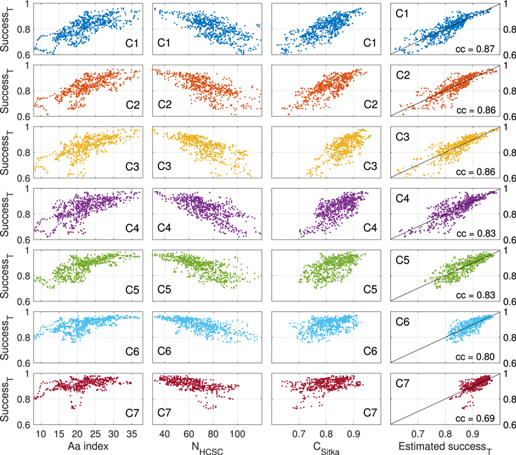
Figure 4. Success of T sectors in seven conglomerates of polarity proxies vs. aa geomagnetic activity index (first column), number of the HCS crossings within the 378 day interval (second column), fraction of coincidences between the analyzed conglomerate and the polarities reconstructed from Sitka magnetic data (third column), and estimated T sector success (forth column; lines indicate perfect match).
Download figure:
Standard image High-resolution imageAn evaluation can alternatively be made considering that the IMF is mostly organized in two or four sectors within one solar rotation, so that the polarity does not change for several consecutive days. The large number of the day-to-day polarity changes, i.e., HCS crossings, during a certain period is a sign of an excessive noisiness. The second column of Figure 4 shows an almost linear relation between successT for the C1–C7 conglomerates and the corresponding number of the HCS crossings. The latter were found within the same 378 day intervals. According to the IMF observed in 1965–2018, the median number of the HCS crossings is 62 per 378 days, while in the reconstructed sector structures C1–C7, the median values are 78, 73, 71, 71, 67, 66, and 62.
In Vokhmyanin & Ponyavin (2016), we have shown that the success rate of the inferred sector structure can also be evaluated by comparison with some reference polarity proxy. In this study, the polarities obtained at Sitka magnetic observatory serve as reference proxy. As was mentioned in Section 2, this station is located in Alaska, and its magnetic data do not correlate with the magnetic field at the European stations, which contribute most to the presatellite polarity proxies. To evaluate the reliability of the T sectors in a chosen conglomerate of the polarity proxies, we compare it with the polarities based on Sitka magnetic data. In the third column of Figure 4, the ratio of coincidences during the 378 days intervals almost linearly corresponds to the T sector success.
Finally, we evaluate the accuracy of the T sectors in each proxy using the following nonlinear regression:
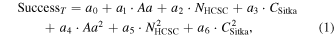
where the variable Aa is the aa index, NHCSC is the number of HCS crossings, CSitka is the fraction of coincidences with the sector structure obtained from Sitka magnetic data, and a1 − 6 are the regression coefficients. The estimated success of negative polarities in each conglomerate of proxies is shown in the last column of Figure 4. The correlation between the actual and estimated values is above 0.8 for C1–C6, and almost 0.7 for C7.
In Figure 5, red curves represent the success rate for T sectors estimated according to Equation (1). Thick black curves indicate the success rate found for each data set by comparison with the observed IMF. All three parameters used for the success reconstruction are available since 1902, when Sitka magnetic station started to operate. For the earlier years, we can use only geomagnetic activity and the number of the HCS crossings as proxies for T sector success,


Figure 5. Estimated reliability of the T sectors for each conglomerate of the polarity proxies. Thick black curves show actual success rates found by comparison with the observed IMF. Red curves are for the success estimated in Equation (1), blue curves show the success estimated in Equation (2), and green curves show the success estimated in Equation (3).
Download figure:
Standard image High-resolution imageIn this case, the success is also evaluated reasonably well. The linear correlation coefficients between actual and reconstructed success values are 0.84, 0.82, 0.81, 0.81, 0.82, 0.79, and 0.67 for the conglomerates C1–C7 in 1965–2018. In Figure 5, these results are shown with blue curves.
To estimate the success before 1868 when there were no aa index measurements, we use the ΔHD index, which is the average absolute hour-to-hour deviation of H and D horizontal geomagnetic components at Helsinki (Nurmijarvi) and Saint Petersburg (Voeikovo) stations. Martini et al. (2016) have shown that such an index based on the variability of the horizontal geomagnetic component is consistent and useful for the geomagnetic studies. On an annual scale, the geomagnetic activity is very similar in different indices, so replacing aa with ΔHD will not affect the evaluation of the T sector reliability,

In this case, the correlation coefficients between the actual and reconstructed success values are 0.85, 0.83, 0.82, 0.82, 0.83, 0.80, and 0.68 for conglomerates C1–C7 in 1965–2018. In Figure 5, this approach is shown with green curves.
The estimated success apparently decreases before 1930, coinciding with the period of low geomagnetic activity, weak IMF intensity, and secular minimum of solar activity. This long-term weakening of the IMF intensity is seen in several reconstructions based on sunspot data, geomagnetic data, and cosmogenic radionuclide data (Svalgaard & Cliver 2010; McCracken & Beer 2015; Owens et al. 2016). The lowest reliability of the inferred polarities is found in the years of deep solar and geomagnetic activity minima in 1856, 1878, and 1901.
It is also possible to verify the conglomerates by checking out the well-known patterns inherent in the IMF sector structure. The first is that the semiannual variation in geomagnetic activity is caused by opposite sectors: the Autumn peak is due to negative IMF polarity, and the Spring peak is due to positive IMF polarity (Russell & McPherron 1973). In Vokhmyanin & Ponyavin (2012), we demonstrate that this is true for the polarities inferred since 1905. Svalgaard et al. (2016) also confirm this for the sector structure in the 19th century. Second, the IMF polarities follow the Rosenberg-Coleman rule: during equinoxes, when the Earth passes above/below the heliographic equator, one might expect more IMF with the polarities of the corresponding solar hemisphere (Rosenberg & Coleman 1969). When the solar dipole is negative (positive), more negative (positive) sectors within the ecliptic are observed in Fall, and more positive (negative) sectors in Spring. This pattern is also inherent to the analyzed conglomerates of the inferred polarities (see Figure 10 in the Appendix). Compliance with these regularities also confirms the reliability of the reconstructed sector structure throughout the study period.
3.3. Correction of the Inferred Fraction of the Negative IMF Polarity
The uncertainty of the reconstructed fractions of the negative IMF polarity comes from (1) the variability of the actual fraction of T sectors (black curve in Figure 2) and (2) from the variability in the combination of the success for T and A sectors (Figure 3(h)). These two factors determine the range of differences between the actual and the reconstructed values (gray dots in Figures 3(a)–(g)). When evaluating the correction term and uncertainty of the T sector fraction in the past, we also have to consider the uncertainty of the estimated success as apparent from the last column of Figure 4.
To simulate the response of Equation (1), we add a random noise with the distribution given by the fitted models (Equation (1)). In Figure 6, colored dots indicate the observed errors versus the actual responses of Equation (1). Here, we combine simulations for the conglomerates C1–C4 and C5–C6, which have a very similar error distribution. The dotted black curves show the 95% confidence range of the errors in the simulated T sector fraction values depending on the simulated successT values. The average errors of the T sector fraction are shown by thick black curves. The tendency of low (high) success points to an underestimated (overestimated) T sector fraction that becomes less steep compared to Figures 3(a)–(g). The average errors and 95% confidence limits were interpolated with quadratic functions (red curves), which are used to calculate additional terms to the original values of the T sector fraction (Figure 2) in the presatellite era. The result is shown in Figure 7 (these data are attached as a supplement in seven separate files for each conglomerate; see Table 3 for the description). Note that in the 19th century, where only C1 and C2 are available, the estimation is made according to Equation (2) back to 1868 (shown with blue curves), and back to 1844 according to Equation (3) (green).

Figure 6. Difference between the actual and reconstructed fraction of T sectors vs. estimated reliability of the negative IMF polarity. The average errors of the simulated data points are shown by thick black curves, and the dotted curves indicate the 95% confidence range. The red curves illustrate the quadratic interpolation.
Download figure:
Standard image High-resolution image
Figure 7. (a–g) Fraction of T sectors according to the conglomerates of the inferred IMF polarities C1–C7 (red curves) and according to the observed IMF (black curve). The fraction values are corrected using the reliability of the T sectors estimated in Equation (1) (red), Equation (2) (blue), and Equation (3) (green). Gray curves show the 95% confidence range. (h) Black curve show the compilation of the most reliable values, shaded areas represent the 95% confidence interval, green areas show sunspot numbers, red canvases on the ascending phases highlight the T sector dominance, blue shows the A sector dominance; "S" indicates the southward shift of the HCS, and "N" indicates the northward shift.
Download figure:
Standard image High-resolution imageTable 3. Description for the Catalogs of the Reconstructed Fractions of T Sectors within 378 day Intervals According to the Sector Structure in Conglomerates C1–C7
| Num | Label | Explanations |
|---|---|---|
| 1 | YYYY | Year of the central date within the 378 day interval |
| 2 | MM | Month of the central date within the 378 day interval |
| 3 | DD | Day of the month of the central date within the 378 day interval |
| 4 | FT | Fraction of T sectors according to the corresponding conglomerate |
| 5 | ST | Estimated fraction of correctly defined T sectors |
| 6 | FT1 | Corrected fraction of T sectors in the corresponding conglomerate |
| 7 | FT2 | Lower boundary for the corrected fraction of T sectors (2.5th percentile) |
| 8 | FT3 | Lower boundary for the corrected fraction of T sectors (15.9th percentile) |
| 9 | FT4 | Upper boundary for the corrected fraction of T sectors (84.1th percentile) |
| 10 | FT5 | Upper boundary for the corrected fraction of T sectors (97.5th percentile) |
Note. Table 3 is published in its entirety in machine-readable format. Here, we show explanations for each column of the table.
Only a portion of this table is shown here to demonstrate its form and content. A machine-readable version of the full table is available.
Download table as: DataTypeset image
Finally, using the observed IMF during 1965–2018 and the most reliable values of the T sector fraction before 1965, we compile total time series describing which of the IMF polarities dominated at the ecliptic. According to the period covered by the spacecraft observations (cycles 20–24), a distinct dominance of the IMF with the polarity of the northern solar hemisphere and thus southward shift (marked with "S") of the HCS was seen in the ascending phase of the solar cycles (Figure 7(h)). During the ascending phase, the HCS is less disturbed by the high-speed solar wind streams, and the N–S asymmetry is clearly seen. We highlight the dominance of the T sectors by red canvases and A sectors by blue curves. In the presatellite era, a northward shift of the HCS is seen in the ascending phase of cycles 10, 15, and 17–19; a southward shift of the HCS is seen in the ascending phase of cycles 9, 11–14, and 16. This result is discussed in detail in the following section.
4. Discussion
It would be useful to compare the N–S asymmetry in the HCS with another long-term data set estimating the hemispheric inequality. Sunspot time series are the longest measurements of the solar activity directly in the northern and southern hemispheres. Observations by Staudacher provided in 1749–1796 were digitized by Arlt (2008, 2009), observations by Schwabe in 1825–1867 were digitized by Arlt (2011) and Arlt et al. (2013), and observations by Spörer in 1868–1874 were processed by Pulkkinen & Tuominen (1998). We also use the RGO, USAF, and NOAA 3 data in 1875–2016.
Figure 8(a) shows the annual number of observation days. Blue bars mark data provided by Staudacher, yellow bars shows data from Schwabe, green bars show data from Spörer, and gray shows data according to the RGO database. Staudacher records are the rarest, and the N–S asymmetry found for this period is of low reliability. Note also that number of reports by Staudacher and Schwabe is modulated by the solar cycle.

Figure 8. (a) Number of observation days per year: blue denotes Staudacher, yellow stands for Schwabe, green shows Spörer, and gray represents RGO. (b) Yearly mean counts of sunspot groups in the hemispheres; blue indicates the northern hemisphere dominance, and red is southern hemisphere dominance. The cycle numbers refer to the Zürich ordering. (c) The thin green curve stands for the N–S asymmetry of the yearly mean sunspot group counts, the thick green curve is a 10 yr moving average, and purple is the long-term mode. Blue canvas highlights the long-term solar activity dominance in the northern hemisphere, and red shows this in the southern hemisphere. (d) The thin gray curve denotes yearly sunspot groups of the entire solar disk. The thick dashed gray and solid black curves are two modes defined by means of the EMD method.
Download figure:
Standard image High-resolution imageThe N–S asymmetry estimation requires group numbers of the northern and southern hemispheres. Unfortunately, the earliest observations are available only for the entire Sun. Figure 8(b) shows the raw yearly mean sunspot counts reported by Staudacher, Schwabe, Spörer, and RGO–USAF/NOAA data. For each data set, hemispheric sunspot group counts are calculated according to the sign of their latitudes. We did not use the normalization between different observers. These factors are reduced by the definition of the N–S asymmetry formula. Due to the lack of normalization, one might notice that the amplitude of cycle 4 is as high as that of cycle 24 and higher than that of cycle 14.
Staudacher did not assign sunspot groups. We manage this by limiting the linear size of a group to 5° in latitude and 10° in longitude. We also tested smaller and larger limits, but the group counts are not significantly affected by these changes. Sunspots with zero latitude were excluded from the analysis.
In Figure 8(b), blue areas denote periods when the group counts in the northern hemisphere are higher than in the southern hemisphere. Otherwise, the difference in counts is shaded red. Although the observations by Staudacher and Schwabe cover the secular maxima, their group counts and the difference between hemispheres is smaller than in the Greenwich records.
In Figure 8(c), the (N − S)/(N + S) asymmetry ratio is shown. N is the yearly group counts in the northern hemisphere and S shows the same in the southern hemisphere. The thin green curve denotes yearly values of the N–S asymmetry, and the thick green curve is a moving 10 yr average. The thick purple curve is the long-term mode extracted from the yearly N–S asymmetry by the empirical mode decomposition method (EMD; Huang et al. 1998). 4 Staudacher records are too short and to little reliable to calculate the average. Blue and red canvas mark the periods when the northern and southern hemisphere dominates in the long term. The amplitude of the N–S asymmetry varies significantly, but the sign of the long-term modes persists through several solar cycles. The long-term hemispheric dominance changes between cycles 9 and 10, between cycles 14 and 15, and in cycle 20.
The hypothesis of the long-term N–S asymmetry is not new. Analyzing solar activity of cycles 8–22, Verma (1992) reported nearly the same intervals of a persistent long-term N–S asymmetry as in Figure 8(c) and proposed that such an asymmetry may have a period of 12 solar cycles and will shift to the northern hemisphere in cycle 25. Analyzing the RGO data, Li et al. (2002) also claimed a 12-cycle periodicity. In contrast, Badalyan & Obridko (2017) reported that the long periods of positive or negative asymmetry obey a Poisson distribution, i.e., correspond to a random process.
The N–S asymmetry according to Staudacher observations should be analyzed taking into account the number of observation days within a year. Yearly mean counts of sunspot groups calculated over a few observations lose reliability. Note that sharp jumps in asymmetry occurred during periods of rare observations. Certainly, the assumption of the long-term N–S asymmetry change near cycle 4 is weak. In addition, the southern dominance is observed only for half of the cycle. The available data suggest that from the maximum of cycle 1 to the maximum of cycle 4, the northern hemisphere commonly dominates. If this is so, the chronology of the constant long-term period of the N–S asymmetry is disrupted. This idea would suggest a sign change near cycles 4 and 5 and would be opposite to the observed sign change. Note that cycle 4 is referred to as unusual. For example, one cycle was suggested to be lost in the beginning of the Dalton minimum (Usoskin et al. 2001, 2002; Zolotova & Ponyavin 2011; Karoff et al. 2015; Nagovitsyn & Pevtsov 2020), and the Gnevyshev & Ohl (1948) rule was violated during this period (Nagovitsyn et al. 2009; Ogurtsov 2012; Tlatov 2013, 2014; Zolotova & Ponyavin 2015).
Figure 8(d) compares periods of persistent hemispheric dominance and long-term variations in solar activity. The thin gray curve denotes yearly mean sunspot groups of the entire solar disk (Svalgaard & Schatten 2016). The thick dashed gray and solid black curves are two modes defined by means of the EMD method. For the observations by Schwabe, Spörer, and RGO, the periods of the northern dominance coincide with the ascending branch of the secular mode, while the southern dominance lies on the descending branch. This result partially confirms the scenario by Waldmeier (1957) for the amplitude asymmetry of the solar activity on the secular scale and results by Vizoso & Ballester (1990). Observations by Staudacher violate the scenario described by the secular mode, but obey the relation with the long-term mode. Cycles 1–3 constitute the ascending branch of the long-term mode, where the northern hemisphere dominates.
The long-term variation is also revealed in the phase shift (or phase asynchrony) of solar activity in the hemispheres (Donner & Thiel 2007; Zolotova et al. 2009; McIntosh et al. 2013; Muraközy 2016) and in the lengths of the butterfly wings (Pulkkinen et al. 1999; Zolotova et al. 2010; Badalyan 2011; Leussu et al. 2016). Hypotheses about the relation of all these different measures of the N–S asymmetry require further investigations.
The HCS N–S asymmetry estimated in this study (Section 3.3) is presented in Figure 9(a). Here, we show the fraction of the positive polarity sectors (1 − NT /Nall) when the solar dipole sign was negative, so that overall, Figure 9(a) shows the fraction of the sectors with the polarity of the southern hemisphere (NS /Nall). The solar dipole is assumed to be negative between consecutive solar magnetic field reversals in odd and even cycles. Since 1907, the years of the dipole reversals (red circles in Figure 9(c)) are defined according to the minimum of polar magnetic fluxes reconstructed by Muñoz-Jaramillo et al. (2012), and since 1976 according to the fluxes observed at the Wilcox Solar Observatory. Before 1907, reversals were defined as the next year after the year of solar activity maximum. Considering the uncertainty of the solar dipole sign within the reversal year, we exclude corresponding data from the consideration.

Figure 9. (a) Fraction of the sectors with the polarity of the southern hemisphere; the moving 5 yr average (thick blue curve) reveals the long-term variation. (b) Long-term variations of the N–S asymmetry in the yearly mean sunspots group counts (green curve), sunspot rotation at 17° latitude (Zhang et al. 2013; black curve), and heliospheric current sheet. (c) Yearly mean total sunspot numbers. The red circles are the years of the dipole reversals.
Download figure:
Standard image High-resolution imageThe thick blue curve denotes a long-term variation found as a 5 yr moving average (Figure 9(a)). The persistent northward shift of the HCS during cycles 15–19 (except for cycle 16) changes to the southward shift in cycles 20–24 in accordance with the long-term N–S asymmetry of sunspot groups. Since the descending phase of cycle 10 to cycle 14, the HCS was coned southward on average.
Hiltula & Mursula (2006) suggested the long-lasting southward shift of the HCS. They consider only several years prior to the solar activity minimum. In Figure 9(a), we take into account the whole interval between two consecutive dipole reversals. Similar long-term variations of the HCS are found if we consider data only during ascending phases (Figure 7(h)). We assume that using these approaches, the northward shift of the HCS during cycles 17–19 would be also seen in the IMF polarities provided by Vennerstroem et al. (2001).
The HCS deflection follows the polar field imbalance (Smith et al. 2000). Thus, it can be compared with the N–S asymmetry of the polar field or polar field fluxes. Muñoz-Jaramillo et al. (2012) used polar facula numbers (Sheeley 2008) observed at Mount Wilson Observatory and calibrated them to the fluxes measured at Wilcox Solar Observatory. According to their results, the northern polar flux strongly dominated within three consecutive solar activity minima (between cycles 17 and 20), in agreement with our conclusions. The southern polar flux dominated during cycle 16 (Muñoz-Jaramillo et al. 2012, Figure 14). The corresponding dominance of the IMF with the polarity of the northern hemisphere is seen in cycle 16 (Figure 9(a)).
The sunspot rotation is known to be anticorrelated with sunspot area (Howard et al. 1984; Hathaway & Wilson 1990): in case of strong mid- and low-latitude magnetic fields, i.e., high sunspot activity, the rotation velocity would be slower. Zhang et al. (2013) studied the differential rotation of active longitudes in 1877–2008 and found an 80–90 yr asymmetry oscillation in antiphase with large sunspot activity. They suggested that the northern hemisphere at 17° reference latitude rotated faster before the 1910s and since the 1970s, while the southern hemisphere was faster in between, in cycles 15–20. We show their results (reversed Figure 5 from Zhang et al. 2013) in Figure 9(b) as a black curve. Note, however, that according to Pulkkinen & Tuominen (1998), the southern hemisphere at 15° was rotating faster in cycles 10–11 and 14–19, and the northern rotated faster in cycles 13 and 20–22.
Long-term variation is also inherent to other indices associated with the nondipolar field. Li et al. (2010) showed that cumulative filament numbers in cycles 16–20 were larger for the northern hemisphere and smaller in cycle 21. Verma (1993, 2000) analyzed several quantities of solar activity, such as sunspot areas, sunspot numbers, solar flares, sudden disappearing filaments, and prominences, and found that the southern hemisphere dominated during cycles 10–14 and 21–23, while the northern hemisphere dominated during cycles 7–9 and 15–20.
Thus, similar long-term N–S asymmetry variations are present in both poloidal (HCS shift and polar fluxes) and toroidal (sunspots, solar activity, and sunspot rotation) solar magnetic field manifestations. In Figure 9(b), we show long-term variations of the HCS deflection (fraction of the polarities from the southern hemisphere minus 0.5), long-term asymmetry in sunspots, and long-term asymmetry in sunspot rotation (Zhang et al. 2013). These quantities do not exactly repeat each other, but represent the same phenomena: dominance of the north around cycles 16–19 (ascending phase of the secular solar cycle) and dominance of the south in cycles 11–14 and 21–24 (descending phase of the secular solar cycle).
According to Figure 9(b), changes in the HCS asymmetry seem to precede the same changes in sunspot asymmetry. However, this has to be investigated with more precise data sets. Bhowmik (2019) suggests that the asymmetry of the polar fluxes at solar cycle minimum corresponds to the total hemispheric activity in the following cycle. The imbalance between northern and southern poloidal magnetic fields that causes the HCS deflection transforms into the asymmetric toroidal fields that manifest themselves through sunspot activity.
Yet the community does not have a generally accepted theory for the origin of the long-term hemispheric asymmetry. Mathematically, it could be expressed as an asynchrony between dipolar and quadrupolar solar dynamo modes, which have different cycle durations (Sokoloff & Nesme-Ribes 1994). For instance, Virtanen & Mursula (2016) show that during cycles 20–22 and cycle 24, the southward shift of the HCS is due to a quadrupole term of the photospheric magnetic field. They also suggest that a stronger southern magnetic field was formed by N–S asymmetric surges of the magnetic flux from the middle latitudes during solar activity maximum.
5. Conclusion
In this paper, we evaluate the HCS N–S asymmetry using IMF polarities reconstructed from geomagnetic variations. We compile seven homogeneous conglomerates of the inferred polarities covering different time periods since 1844. We estimate the reliability of the negative IMF polarities (T sectors) for all data sets in the presatellite era, which is mostly 80 to 90% correct daily polarities within 378 day intervals. Lower success is mostly found in the years of low solar and geomagnetic activities and degrades in the past due to the lower number of magnetic stations. We found that during intervals with low reliability of the negative IMF polarity, the fraction of T sectors tends to be underestimated and vice versa for higher reliability. This relation was used to correct the inferred T sector fraction in the presatellite era.
In accordance with spacecraft IMF observations, we found more sectors with the polarity of the northern hemisphere during cycles 20–24, indicating a southward shift of the HCS. This asymmetry is especially visible in the ascending phase of solar activity. We found that the HCS was on average coned northward at the beginning of cycle 10 and from the maximum of cycle 15 to cycle 19 (except for cycle 16). The same dominance of the northward polar field with the exception of cycle 16 is seen in the reconstructed polar fluxes (Muñoz-Jaramillo et al. 2012). For the earlier cycles, the amplitude of the long-term HCS asymmetry decreases and the uncertainty increases. However, there is evidence of a southward shift of the HCS in the ascending phase of cycle 9 and cycles 11–14.
We also evaluate the sunspot group N–S asymmetry using the observations in 1749–1796 by Staudacher and in 1825–1874 by Schwabe and Spörer as well as RGO, USAF, and NOAA data in 1875–2016. The long-term mode of the N–S asymmetry of sunspots reveals that the northern hemisphere dominated in cycles 2–3, 7–9, and 15–20, while the southern hemisphere activity was stronger in cycles 4, 9–14, and 21–24.
The same long-term N–S asymmetry is also seen in other manifestations of the solar magnetic field (Verma 2000; Li et al. 2010; Zhang et al. 2013). The consistent pattern of the amplitude asymmetry proposed by Waldmeier (1957) might be valid: during the ascending phase of the secular cycle, the northern activity dominates, and in the descending phase, the southern activity is stronger. The origin of this relation is not clear, and because the available proxies cover only one and a half secular cycles, we cannot conclude that the long-term asymmetry variation is a regular phenomenon. However, our findings emphasize the importance of the N–S asymmetry factor in the development of the solar dynamo models.
This paper was motivated by and would not appear without the guidance of Dmitri Ponyavin. The authors thank Rainer Arlt from the Astrophysikalisches Institut Potsdam for the digitized Staudacher and Schwabe sunspot observations (old.aip.de/Members/rarlt/sunspots). RGO and USAF/NOAA sunspot data were obtained from sidc.oma.be/silso/datafiles. Spacecraft observations of the IMF were obtained from the OMNI database. The Aa geomagnetic index is calculated and made available by ISGI Collaborating Institutes from data collected at magnetic observatories. We thank the involved national institutes, the INTERMAGNET network, and ISGI (isgi.unistra.fr). We also thank the referees for their helpful, critical comments and their assistance in evaluating this paper.
The reported study was funded by the Russian Science Foundation according to the research project 19-72-00053.
Appendix
Figure 10 demonstrates the presence of the semiannual variation of the dominant IMF polarity, the so-called Rosenberg-Coleman rule, in the conglomerates C1–C5. See the end of Section 3.2 for details.

Figure 10. Rosenberg-Coleman rule in five conglomerates of the inferred IMF polarities calculated as the difference between the fraction of negative sectors (NT /Nall) in Spring and Fall; thick black curves show this effect according to the observations. The data are approximated with sine functions (dashed curve), which are presented in each panel. The dotted vertical lines indicate solar activity minima; the numbering of solar cycles is indicated at the top. More negative (positive) sectors are seen within the minima between even and odd cycles.
Download figure:
Standard image High-resolution image
Footnotes
- 3
Royal Greenwich Observatory, United States Air Forces, and National Oceanic and Atmospheric Administration.
- 4
The EMD method provides a set of modes and the nondecomposable residual. The sum of the modes and the final residual is equal to the original signal. In Figure 8(d), we show two low-frequency modes extracted from the yearly sunspot groups, called "long-term" and "secular", for simplicity.