


Abstract
We present K-band interferometric observations of the PDS 70 protoplanets along with their host star using VLTI/GRAVITY. We obtained K-band spectra and 100 μas precision astrometry of both PDS 70 b and c in two epochs, as well as spatially resolving the hot inner disk around the star. Rejecting unstable orbits, we found a nonzero eccentricity for PDS 70 b of 0.17 ± 0.06, a near-circular orbit for PDS 70 c, and an orbital configuration that is consistent with the planets migrating into a 2:1 mean motion resonance. Enforcing dynamical stability, we obtained a 95% upper limit on the mass of PDS 70 b of 10 MJup, while the mass of PDS 70 c was unconstrained. The GRAVITY K-band spectra rules out pure blackbody models for the photospheres of both planets. Instead, the models with the most support from the data are planetary atmospheres that are dusty, but the nature of the dust is unclear. Any circumplanetary dust around these planets is not well constrained by the planets' 1–5 μm spectral energy distributions (SEDs) and requires longer wavelength data to probe with SED analysis. However with VLTI/GRAVITY, we made the first observations of a circumplanetary environment with sub-astronomical-unit spatial resolution, placing an upper limit of 0.3 au on the size of a bright disk around PDS 70 b.
Export citation and abstract BibTeX RIS

Original content from this work may be used under the terms of the Creative Commons Attribution 4.0 licence. Any further distribution of this work must maintain attribution to the author(s) and the title of the work, journal citation and DOI.
1. Introduction
The process of transforming the dust around stars into mature planetary systems is complex and multifaceted. The initial stages of planet formation are mostly hidden from observations as planets grow from small embryos to large cores to natal protoplanets through processes such as streaming instability, planetesimal accretion, or even gravitational instability (Bodenheimer 1974; Pollack et al. 1996; Youdin & Goodman 2005). For gas giants like our own Jupiter, after they have grown large enough to undergo runaway growth, we can begin to indirectly observe them as they carve out gaps and excite density waves in the circumstellar disk as they orbit the star (e.g., van der Marel et al. 2013; Casassus et al. 2013; Pérez et al. 2014; ALMA Partnership et al. 2015; Andrews et al. 2018). During this process, the dynamical interactions between the protoplanet and the disk can cause the planet to migrate in the disk (Lin & Papaloizou 1986; Ward 1997; Duffell et al. 2014). In systems with multiple protoplanets, interactions with the disk and planets can excite eccentricities, cause dynamical instabilities, or lock the planets in resonance (Dong & Dawson 2016). As the protoplanets accrete more material, they grow to detectable levels, and emerge from the shroud of dust and gas that obscured them from direct observations (Zhu 2015; Ginzburg & Chiang 2019a; Szulágyi et al. 2019). After the circumstellar gas disk clears, the gas giant planet formation process is effectively over, leaving behind the many planetary systems we see today.
Catching a glimpse of protoplanets in the process of forming is difficult due to circumstellar and circumplanetary dust shrouding them at the earliest times (Zhu 2015; Szulágyi et al. 2019). The distances of nearby systems young enough to still be undergoing planet formation (e.g., Boccaletti et al. 2020) are ⪆ 100 pc, making it difficult to spatially resolve them from their circumstellar disks using single-dish 8–10 m telescopes. For both of these reasons, the ability to identify and characterize young protoplanets currently have been limited. Several protoplanets have been reported (Kraus & Ireland 2012; Quanz et al. 2013; Biller et al. 2014; Reggiani et al. 2014; Currie et al. 2015; Sallum et al. 2015), but have had their classification questioned (Thalmann et al. 2015; Follette et al. 2017; Rameau et al. 2017; Ligi et al. 2018; Mendigutía et al. 2018).
Out of all the sources reported, only the two sources around PDS 70 are undeniably protoplanets in nature. Like many other protoplanet candidates, the star PDS 70 harbors a circumstellar disk with features such as a large gap that may be due to planets in the system (Dong et al. 2012; Hashimoto et al. 2012; Hashimoto et al. 2015). As part of the SHINE exoplanet survey (Chauvin et al. 2017; Vigan et al. 2020), PDS 70 b was discovered clearly inside the gap and imaged at multiple wavelengths unlike other protoplanet candidates, making it easy to rule out confusion with circumstellar disk features (Keppler et al. 2018; Müller et al. 2018). PDS 70 c could not be confidently identified as a protoplanet initially due to the fact it appeared adjacent to the rim of the circumstellar disk in projection. It was discovered with Hα imaging (Haffert et al. 2019), which took advantage of the fact that only protoplanets and their host stars that are actively accreting material are hot enough to emit strong atomic hydrogen emission lines. The protoplanet nature of both planets was confirmed by their strong Hα detections that imply mass accretion rates of at least 10−8 MJup/yr (Wagner et al. 2018; Haffert et al. 2019). Assuming their orbits are coplanar with the circumstellar disk that has been well characterized in the near-infrared and millimeter wavelength (Keppler et al. 2018, 2019; Francis & van der Marel 2020), the planets are near the 2:1 period commensurability (Haffert et al. 2019; Wang et al. 2020). Dynamical studies have shown that having these two planets in mean-motion resonance (MMR) would be stable and could create the disk features we see (Bae et al. 2019; Toci et al. 2020). However, with a short orbital arc and uncertainties of several mas, their exact orbit remains uncertain (Wang et al. 2020).
Owing to their protoplanetary nature, it is currently inconclusive what emission we are seeing from the planets and their circumplanetary environments. Current low-resolution spectroscopy and photometry from 1 to 5 μm point to emission that is very dusty with only one tentative water absorption feature for PDS 70 b (Müller et al. 2018; Christiaens et al. 2019b; Haffert et al. 2019; Mesa et al. 2019; Wang et al. 2020; Stolker et al. 2020). The cause of the dusty spectrum could be due to high-level hazes in the atmosphere, the accretion of material onto the planet, or a circumplanetary or circumstellar disk obscuring the planet, with recent analysis favoring accreting material being responsible (Wang et al. 2020; Stolker et al. 2020). The spectral characterization of PDS 70 c has been especially challenging, requiring high angular resolution imaging and disk modeling to properly extract photometry from the protoplanet (Haffert et al. 2019; Mesa et al. 2019; Stolker et al. 2020; Wang et al. 2020). Despite having a relatively large wavelength coverage, the emission from both planets was found to still be consistent with a single blackbody, with no support from the data for using more sophisticated models (Wang et al. 2020; Stolker et al. 2020). However, it is unlikely that the true emission from these protoplanets are blackbodies. As these planets are accreting, there also should be dust in their circumplanetary environments. There has been tentative evidence for a circumplanetary disk (CPD) around PDS 70 b with K- and M-band excess (Christiaens et al. 2019a; Stolker et al. 2020), and a significant ALMA detection of dust at the location of PDS 70 c (Isella et al. 2019).
Long-baseline optical interferometry allows us to combine multiple single-dish telescopes together to achieve an order of magnitude boost in angular resolution, important for discerning protoplanets from circumstellar and circumplanetary dust (Wallace & Ireland 2019). Recently, the GRAVITY interferometer at VLTI made the first direct detection of an exoplanet with optical interferometry using its pioneering phase-referenced dual-field mode (Gravity Collaboration et al. 2019). This mode has shown GRAVITY can achieve astrometric precisions down to 50 μas and obtain high signal-to-noise K-band spectra of exoplanets at R ∼ 500 (Gravity Collaboration et al. 2020; Mollière et al. 2020; Nowak et al. 2020).
In this work, we will leverage the superior angular resolution of GRAVITY combined with its ability to distinguish coherent and incoherent emission to study the PDS 70 protoplanets. In Section 2, we describe the observations made of PDS 70 b and c as well as its host star, the data reduction, and spectral calibration. We then fit the orbit of both planets and make dynamical mass constraints based on stability arguments in Section 3. In Section 4, we fit multiple atmospheric models, explore the evidence for extinction and circumplanetary disk emission, discuss the nature of the photospheric emission from these protoplanets, and place limits on Brγ accretion signatures. We also use the long-baseline data from GRAVITY to attempt to resolve the circumplanetary environment in Section 5. Finally we offer some concluding thoughts in Section 6.
2. Observations and Data Reduction
2.1. GRAVITY Observations
The observations were carried out using the GRAVITY instrument (Gravity Collaboration et al. 2017) on the VLTI using the four Unit Telescopes (UT). The log of the observations are given in Table 1. Atmospheric conditions ranged from very good (atmospheric coherence time τ0 = 20 ms) to average (τ0 ≈ 2 ms). The first observation, in 2018, is a classical interferometric observation of the star (PI M. Benisty, ID 0101.C-0281). The 2019 observations were obtained as a backup of the AGN large program (PI E. Sturm, ID 1103.B-0626, for PDS 70 b), and from director discretionary time (PI A. Vigan, ID 2103.C-5018, for PDS 70 c). Last, the 2020 observations were obtained as part of the ExoGRAVITY large program (PI S. Lacour, ID 1104.C-0651).
Table 1. Log of the Observations
| Target | Date | UT Time | Resolution | Nexp/NDIT/DIT a | Airmass | τ0 | Seeing | |
|---|---|---|---|---|---|---|---|---|
| Planet | Star | |||||||
| PDS 70 A | 2018-06-25 | 01:13:21–01:30:12 | MEDIUM | ⋯ | 3/30/10 s | 1.05–1.07 | 2.0–2.7 ms | 0.55–0.80'' |
| HD 124058 | 2018-06-25 | 01:44:45–02:01:42 | MEDIUM | ⋯ | 3/30/10 s | 1.07–1.09 | 2.0–2.7 ms | 0.55–0.80'' |
| PDS 70 b | 2019-07-16 | 00:09:49–01:01:39 | MEDIUM | 3/12/60 s | 3/64/1 s | 1.07–1.15 | 1.7–2.3 ms | 0.87–1.32'' |
| PDS 70 b | 2020-02-10 | 07:09:28–08:38:48 | MEDIUM | 3/8/100 s | 6/8/10 s | 1.05–1.21 | 11.0–21.4 ms | 0.61–0.73'' |
| PDS 70 c | 2019-07-19 | 00:11:46–01:19:17 | LOW | 7/16/30 s | 8/64/1 s | 1.08–1.21 | 3.7–5.5 ms | 0.72–1.2'' |
| PDS 70 c | 2020-02-10 | 07:29:01–09:13:45 | MEDIUM | 4/8/100 s | 6/8/10 s | 1.05–1.21 | 11.0–21.4 ms | 0.61–0.73'' |
Note.
a Nexp is the number of exposures; NDIT is the number of sub-integrations; DIT is the detector integration time. The three values can be multiplied together for the total integration time.Download table as: ASCIITypeset image
The 2018 observations were carried out using the single-field on-axis mode. On-axis means the beam splitter was used (Pfuhl et al. 2014), therefore sending 50% of the flux to the fringe tracker (Lacour et al. 2019) and 50% on the science channel. Single-field means the fringe tracker and the science fibers observed the same object: in this case, the star PDS 70 A. The observations were followed by observations of the calibrator HD 124058. The reduction of this data set was standard using the ESO GRAVITY pipeline 27 (Lapeyrere et al. 2014).
The observations of the exoplanets used the dual-field on-axis mode. Dual-field means the fringe tracker and the science fibers observed different objects. Thanks to the splitter, the fringe tracker observed the star for phase referencing, and the science fibers observe the planet. Non-common path phase aberrations were calibrated by interleaving the observation of the planet with single-field on-axis observations.
2.2. Reduction of Relative Astrometry
The coherent flux was extracted following a standard procedure with the ESO GRAVITY pipeline. From this first step, we obtain Vonplanet(b, t, λ) and Vonstar(b, t, λ), the coherent flux observed on the star and the planet as a function of baseline b, time t, and wavelength λ.
The removal of stellar contamination was performed during a second step. The computation is described in detail in Appendix A of Gravity Collaboration et al. (2020). The code is available as a Python library developed by our team. 28 The main objective of the algorithm is to calculate R(λ, b, t), the ratio of the uncontaminated coherent flux between the star and planet:

where Vstar(b, t, λ) and Vplanet(b, t, λ) are the coherent flux of both objects in the absence of stellar speckle. The additional term γ comes from the fact that the science fiber is not exactly positioned at the location of the target in the focal plane (see Appendix A). The astrometry was obtained from the argument of R, the ratio of the coherent flux:

in which (u,v) are the coordinates in the frequency domain and (ΔR. A.,ΔDecl. ) are the sky-coordinates of the planet relative to the star.
The values, obtained by χ2 minimization, are given in Table 2. The error bars given here correspond to the precision of the measurement. They are estimated from the scatter of the astrometric values (between each file, or by splitting the files into independent measurements). The typical precision is 100 μas. The systematic errors, which are ultimately limiting the accuracy of the astrometry, are theoretically smaller. They were estimated to be 16.5 μ (Lacour et al. 2014).
Table 2. Relative Astrometry of PDS 70 b and c
| MJD | ΔR. A. | ΔDecl. | σΔR.A. | σΔDecl. | ρ | |
|---|---|---|---|---|---|---|
| (days) | (mas) | (mas) | (mas) | (mas) | ⋯ | |
| b | 58680.032 | 102.61 | −139.93 | 0.09 | 0.24 | 0.39 |
| b | 58889.341 | 104.70 | −135.04 | 0.09 | 0.11 | −0.89 |
| c | 58683.034 | −214.95 | 32.22 | 0.13 | 0.13 | 0.28 |
| c | 58889.353 | −214.30 | 27.19 | 0.07 | 0.16 | −0.72 |
Note. Due to the interferometric nature of the observations, a correlation coefficient ρ is required to properly describe the confidence intervals, which are not aligned on the sky coordinates. The covariance matrix can be reconstructed using  and
and  on the diagonal, and ρ
σΔR.A.
σΔDecl. off-diagonal.
on the diagonal, and ρ
σΔR.A.
σΔDecl. off-diagonal.
Download table as: ASCIITypeset image
2.3. Reduction of Spectra and Calibration
The coherent fluxes Vstar(b, t, λ) and Vplanet(b, t, λ) are not normalized and therefore include the shape of the spectrum. To extract the spectrum Fplanet(λ), we assumed the planet to be unresolved. The amplitude of coherent flux of the planet is then equal to the planetary flux:

with the phase derived from the astrometry obtained as described in the previous section.
The star itself has an angular size much smaller than 0.1 mas and therefore was not resolved by our observations. However, the visibilities are still below 1 because the interferometer did partially resolve the hot inner disk:

where Jstar(b, t, λ) is the visibility drop due to resolving the central source (star and inner disk). Hence:

The notation ![]()
![]() corresponds to the mean notation: the coherent flux ratio is averaged over b and t. The injection efficiencies γstar and γplanet are real numbers between 0 and 1, where 1 is the theoretical maximum. The value of γplanet was nearly 1 for most epochs except for the first epoch of PDS 70 c when we did not know the precise position of the planet. During this observation, the fiber was pointing 16.5 mas away from the planet, which gave an injection efficiency of ρ = 0.84. The calculation of this term is given in Appendix A.
corresponds to the mean notation: the coherent flux ratio is averaged over b and t. The injection efficiencies γstar and γplanet are real numbers between 0 and 1, where 1 is the theoretical maximum. The value of γplanet was nearly 1 for most epochs except for the first epoch of PDS 70 c when we did not know the precise position of the planet. During this observation, the fiber was pointing 16.5 mas away from the planet, which gave an injection efficiency of ρ = 0.84. The calculation of this term is given in Appendix A.
To obtain Jstar(b, t, λ), we used the observation of PDS 70 A, calibrated by the star HD 124058 (assuming a diameter for the calibrator of 0.136 ± 0.002 mas). The obtained visibilities are shown in Figure 1. They are mostly consistent with a single constant:

The value of the constant does depend on the normalization of the stellar flux. We found that 94% ± 1% of the flux on-axis of the star is unresolved, independent of baseline. That is, 6% of the flux came in excess emission from the hot inner circumstellar disk that is resolved with GRAVITY. An inner circumstellar disk has been predicted from SED analysis (Dong et al. 2012; Hashimoto et al. 2012; Long et al. 2018), detected in scattered light (Keppler et al. 2018; Mesa et al. 2019), and resolved in the millimeter wavelength (Francis & van der Marel 2020).

Figure 1. Plot of the visibilities of PDS 70 A. The dashed line is the average of the visibility, equal to 94% ± 1%. The inset panel represents the u–v coverage of the observations.
Download figure:
Standard image High-resolution imageBecause the inner disk is resolved, we cannot simply use the 2MASS K-band photometry of the system (Cutri et al. 2003) to normalize the stellar model of the star to calibrate the planetary spectra, since it would include excess emission from the circumstellar disk, which is not part of Fstar(λ). Fortunately, the combined scattered light and thermal emission from the inner disk at shorter wavelengths contributes ≲5% of the total flux from the system (Dong et al. 2012), comparable to the 1σ errors on the stellar photometry. Therefore, we used a BT-NextGen stellar atmosphere (Allard et al. 2012) determined from a joint evolutionary-atmospheric model fit to literature optical and near-infrared photometry using the procedure described in Wang et al. (2020). We did not impose a prior on the effective temperature as in Wang et al. (2020), but all other aspects of the fit were the same. From the resulting posterior distributions of the fitted and derived parameters, we measured an age of 8 ± 1 Myr, a mass of 0.88 ± 0.02 M⊙, an effective temperature of  K (higher than the spectroscopically derived value of 3972 ± 36 K; Pecaut & Mamajek 2016), and a surface gravity of
  [dex]. The mass estimated from SED fitting is significantly higher than previous literature estimates from SED fitting (0.76 ± 0.02 M⊙; Müller et al. 2018), but in better agreement with the dynamical mass estimates from circumstellar disk modeling (0.875 ± 0.03 M⊙; Keppler et al. 2019) and from the orbit fits presented in Section 3. A synthetic stellar spectrum was computed by randomly drawing 200 samples from the Markov Chain Monte Carlo (MCMC) chain, taking the median and standard deviation of the flux at each wavelength as the adopted spectrum and corresponding uncertainties, respectively. We used this spectrum as the spectrum of the star (Fstar) to calibrate our planet spectra. The statistical uncertainties in the model stellar spectrum are much lower than the uncertainties on the planetary spectra, but do not include any estimate of systematic errors in the stellar models.
Comparing our stellar model to the 2MASS K-band photometry, we also measured a significant K-band excess of 14% ± 3%, caused by emission from circumstellar material close to the star. This is much greater than the 6% excess emission resolved by GRAVITY. As the stellar variability is dominated by the rotation modulation of the star (Thanathibodee et al. 2019), it is unlikely to be responsible for this disagreement, as the photometric measurements used in the stellar SED fit should average over this variability. Rather, the GRAVITY observations probe spatial scales of 0.2–0.5 au, which are right in the middle of the spatial extent of the inner disk based on models from Dong et al. (2012) and Long et al. (2018). The remaining ∼8% could be emitted closer in to the star where it is not resolved by GRAVITY, or further out at larger spatial scales that are outside the field of view of GRAVITY (∼50 mas). We did not see significant change in the visibilities over the baselines observed, indicating the emission must be significantly closer in or significantly further out. Inner disk models have the inner edge of the disk at 0.05 au so there could be emission that is a factor of ∼3 closer in (Dong et al. 2012; Long et al. 2018). On the other hand, Keppler et al. (2018) detected the inner disk in polarized light with VLT/SPHERE and found the inner disk could be extended out to 20 au, and Francis & van der Marel (2020) found an outer cutoff of 10 au at millimeter wavelengths with ALMA. This also agrees with disk-modeling analysis that found the inner disk to end at 15 au (Long et al. 2018). Any emission outside of 6 au would not have been seen by GRAVITY (would not couple into the single mode fibers). The location of the emission affects our photometric calibration as emission at larger separations do not need to be included in Fstar whereas emission unresolved by GRAVITY needs to be included in Fstar, which ultimately changes the absolute brightness of the planets. Without further information at the moment, we assumed that half of the remaining 8% excess emission comes from the star. For simplicity, we assumed that it has the same spectrum as the star, so we essentially multiplied our model stellar spectrum by 1.04. A 4% change is already much smaller than the 1σ uncertainties on the planet spectra, so the exact scale factor and spectral shape of the excess dust emission should negligibly affect our results.
Since the star is young and accreting with clear Hα emission (Thanathibodee et al. 2019), line emission from the star could affect the calibration of the planetary spectra. However, the stellar Paβ line has not been detected (Long et al. 2018). Given that the Brγ line is expected to be even weaker, and given that it should be unresolved, the impact of the Brγ line on a single spectral element of our planetary spectra should be negligible given the relatively large error bars of a single spectral channel (∼15% of the total flux). Similarly, Long et al. (2018) did not find appreciable CO line emission in the K-band, which too should be unresolved in our data, and thus have a negligible impact on our spectrum. Thus, we concluded that our omission of emission lines in our model stellar spectrum is a reasonable approximation.
With the coherent flux ratio R(λ, b, t) and this model spectrum of the star Fstar(λ) scaled by 1.04, Equation (5) gave us the spectra for both planets. The resulting spectrum as well as the uncertainties are plotted in Figure 2.

Figure 2. GRAVITY K-band spectra of PDS 70 b (left in blue) and PDS 70 c (right in red). In both panels, The points denote the estimated flux in each spectral channel in MEDIUM resolution mode. The darker and lighter shaded regions denote the 1σ and 2σ confidence intervals of the MEDIUM resolution data, accounting for the estimated correlation between neighboring spectral channels. For PDS 70 b, both epochs of data were combined together to create a single spectrum. For PDS 70 c, the LOW resolution epoch is plotted separately as the white squares with black error bars.
Download figure:
Standard image High-resolution image2.4. Reanalysis of SPHERE IFS PDS 70 c Data
We also reanalyzed the SPHERE IFS data on PDS 70 c published in Mesa et al. (2019). Specifically, we reanalyzed the data from 2018-02-24, which were obtained in exquisite conditions (0.40'' seeing). The data were acquired with SPHERE (Beuzit et al. 2019) in its IRDIFS-EXT mode where IFS (Claudi et al. 2008) and IRDIS (Dohlen et al. 2008) observe in parallel, with IFS covering the YJH bands and IRDIS in K1 and K2 band (Vigan et al. 2010). The data were collected with the apodized pupil Lyot coronagraph (Carbillet et al. 2011; Guerri et al. 2011) in its N_ALC_YJH_S configuration optimized for the H band. The raw data were preprocessed using the vlt-sphere 29 open-source pipeline (Vigan 2020) to produce calibrated (x, y, λ) data cubes of coronagraphic images and off-axis reference PSFs.
Stellar PSF subtraction and spectral extraction of PDS 70 c was done using pyKLIP version 2.1 (Wang et al. 2015). We used angular differential imaging (ADI; Liu 2004; Marois et al. 2006) and spectral differential imaging (SDI; Sparks & Ford 2002) to build up a model of the stellar PSF. We used any frame where PDS 70 c moved by one pixel due to ADI and SDI to calculate the principal components to model the star. We used the first 10 principal components, as this gave us the best signal-to-noise on the planet. We used the forward modeling framework described in Pueyo (2016) and Greenbaum et al. (2018) to measure the spectrum of PDS 70 c. We injected eight simulated planets at the same separation but at different azimuthal positions as PDS 70 c, measured their spectra in the same way, and used the scatter in their measured spectra to estimate the uncertainties on the spectrum of PDS 70 c.
Due to the fact the planet is adjacent to the edge of the circumstellar disk, there is concern that the spectral extraction is biased by the disk even with forward modeling. To assess this, we injected five simulated planets at similar separations as PDS 70 c but at other azimuthal positions in the image where the simulated planets would be adjacent to the disk edge and computed the average bias in the flux after spectral extraction. We found and corrected for biases that were at most the size of the 1σ uncertainty of each spectral channel. We also verified that the scatter in flux between these five planets is consistent at the 20% level with the uncertainty we estimated for PDS 70 c in the previous paragraph. In both cases, the errors in the spectral measurements are dominated by the low signal-to-noise of the planet, and not by systematics due to the presence of disk signal.
We found that PDS 70 c is only detected in the last 12 spectral channels of the IFS data (i.e., H-band). Unlike Mesa et al. (2019), the Y- and J-band spectra are consistent with non-detections, and the scatter we measured at those wavelengths is due to noise. We note that the PDS 70 c spectrum from Mesa et al. (2019) only significantly deviates from their median spectrum of the circumstellar disk in the H-band (see their Figure 5c), which may indicate their PDS 70 c spectrum at the Y and J bands are contaminated by the disk. Our measured spectrum appears to be less affected by the disk likely because we used a more aggressive stellar PSF-subtraction routine that filtered out more disk signal. We also found larger uncertainties per spectral channel on average. Our extracted spectrum of PDS 70 c is plotted in Figure 3. Both reductions have indications of correlated noise, as neighboring spectral channels have less scatter than the error bars would imply for uncorrelated spectral channels.

Figure 3. Reanalysis of the PDS 70 c SPHERE IFS spectrum. The dark gray circles are the spectral channels extracted in this work, whereas the light gray squares are from Mesa et al. (2019). We found larger error bars per spectral channel and did not detect the planet short of the H-band.
Download figure:
Standard image High-resolution image3. Orbital Dynamics
3.1. Orbit Fitting
With only two epochs of GRAVITY measurements for each planet, we were able to constrain the positions and velocities of PDS 70 b and c with 100 μas precision (see Table 2, but the accelerations and ultimately the orbital elements of the planet are still limited by the precision of astrometry from single-dish telescopes. We supplemented the GRAVITY astrometry with imaging astrometry from Müller et al. (2018), Mesa et al. (2019), Haffert et al. (2019), and Wang et al. (2020) (see Table 8 in Appendix B).
To define the orbit, we used the following orbital parameters: semimajor axis (a), eccentricity (e), inclination (i), argument of periastron (ω), longitude of the ascending node (Ω), epoch of periastron in units of fractional orbital period (τ), system parallax, and the component masses of each body (Blunt et al. 2020). We defined the orbital elements for each planet in Jacobi coordinates as they vary less when accounting for the effects of multiple planets (see next paragraph). The reference epoch for τ for both planets was MJD 55,000 (2009-06-18). To keep the orbits realistic, we used the same priors as Wang et al. (2020) to impose PDS 70 b and c have non-crossing orbits as well as near coplanarity of the planets and circumstellar disk. We rejected all orbits for which periastron of PDS 70 c is inside of apastron of PDS 70 b. We also applied a Gaussian prior centered at 0 with a standard deviation of 10° on the coplanarity of planet b with the disk, planet c with the disk, and planet b with planet c. We fixed the disk plane to i = 128 3 (equivalent to i = 517 but for clockwise orbits) and PA = 1567 based on Keppler et al. (2019) measurements of the outer disk. The only prior we changed is the one on the stellar mass: we used a Gaussian prior centered at 0.88 M⊙ with a standard deviation of 0.09 M⊙ based on our stellar SED fit in Section 2.3 but with 10% errors to account for model systematics. All our priors are listed in Table 3.
Table 3. Orbital Parameters for PDS 70 b and c
| Orbital Element | Prior | Near-Coplanar | Dynamically Stable |
|---|---|---|---|
| ab (au) | LogUniform(1, 100) a |

|

|
| eb | Uniform(0, 1) a |

|

|
| ib (°) |
 b
b
|

|

|
| ωb (°) | Uniform(0, 2π) |

|

|
| Ωb (°) | Uniform(0, 2π) b |

|

|
| τb | Uniform(0, 1) |

|

|
| ac (au) | LogUniform(1, 100) a |

|

|
| ec | Uniform(0, 1) a |

|

|
| ic (°) |
 b
b
|

|

|
| ωc (°) | Uniform(0, 2π) |

|

|
| Ωc (°) | Uniform(0, 2π) b |

|

|
| τc | Uniform(0, 1) |

|

|
| Parallax (mas) |
 (8.8159, 0.0405) (8.8159, 0.0405) |

|

|
| Mb (MJup) | Uniform(1, 15) |

|

|
| Mc (MJup) | Uniform(1, 15) |

|

|
| M* (M⊙) |
 (0.88, 0.09) (0.88, 0.09) |

|

|
Notes. The orbital parameters used here are defined in Blunt et al. (2020) and are in Jacobi coordinates. For each parameter, the median value of the posterior is listed, with superscript and subscript describing the 68% credible interval (95% credible interval in parentheses).
a Additional prior on periastron of c is larger than apastron of b. b Additional Gaussian prior on the coplanarity of b, c, and the disk.Download table as: ASCIITypeset image
We are sensitive to perturbations on the visual orbit of one of the planets around the star due to the other planet. Essentially, our visual orbits are defined by the relative separation between the planet and the star. A second planet, to first order, perturbs the star's position and causes the measured distance between the first planet and the star to change, creating epicycles in the visual orbit (note that this effect is different from direct planet–planet gravitational interactions, which we will not consider and are much smaller in amplitude). We followed the prescription defined in Brandt et al. (2020) where only the perturbations of inner planets are accounted for. Thus, the visual orbit of PDS 70 c relative to the star is sensitive to the orbit and mass of PDS 70 b, but not the other way around. For a Jupiter-mass planet at 20 au, the peak-to-valley amplitude of this perturbation is 400 μas. To properly model the GRAVITY astrometry, we needed to account for this effect. However, we note that with only two GRAVITY epochs per planet, we did not constrain the masses. Simply, the orbital elements we inferred would have been different if we assumed the planets were massless rather than Jovian mass. In this work, we added uniform priors on planet mass between 1 and 15 Jupiter masses for each planet. Even though recent work (e.g., Stolker et al. 2020; Wang et al. 2020) inferred masses closer to 1 MJup than 15 MJup, we purposely extended the prior range to higher masses to assess if we could rule out high-mass solutions via dynamical stability arguments.
The orbital parameters were inferred by Bayesian parameter estimation using an unreleased version of the orbitize! package with commit id 83356d9 (Blunt et al. 2020), which uses the parallel-tempered affine-invariant sampler ptemcee (Foreman-Mackey et al. 2013; Vousden et al. 2016). This version of orbitize! automatically handles the covariances of the uncertainties in R.A. and decl. that result due to the u–v coverage of the observations. We ran the sampler using 20 temperatures, 1000 walkers per temperature, and 100,000 steps per walker. Convergence was assessed by visual inspection of the walker chains, and by checking that we ran the sampler for at least 100 autocorrelation times. We also accounted for the perturbations on the visual orbits of each planet due to the other planet in the system as described in the previous paragraph. The posterior was formed using the last 40,000 steps from each walker at the lowest temperature. The visual orbit for PDS 70 b is plotted in Figure 4 and the posterior credible intervals (CIs) are listed in Table 3.

Figure 4. Orbits of PDS 70 b and c projected onto the sky. On the left, 100 orbits randomly drawn from the posteriors are plotted in blue and red for PDS 70 b and c, respectively, and measured astrometry from imaging (does not include GRAVITY measurements) are plotted in black. On the center and right are zoomed-in versions of the same plot showing the GRAVITY astrometry for PDS 70 b and c respectively. The tilted error bars in the GRAVITY data represent the principal axes of the error ellipse.
Download figure:
Standard image High-resolution imageWith the new GRAVITY data, we constrained the semimajor axis of PDS 70 b (ab
) to ±2 au (95% credible interval), but ac
to only ±5 au for the same credible interval. Perfectly circular orbits for PDS 70 b are disfavored by the current data whereas PDS 70 c is consistent with circular orbits. The period ratio of PDS 70 c to PDS 70 b is  (68% credible interval;
  for the 95% credible interval), putting it near the 2:1 mean-motion resonance (MMR) as has been proposed by Haffert et al. (2019) and Bae et al. (2019). For the first time, we are able to strongly disfavor all other first-order mean-motion resonances such as the 3:2 and 4:3 MMR. Given these planets are thought to be Jovian mass (Stolker et al. 2020; Wang et al. 2020), if they are locked in MMR, it would likely require the strength of a first-order resonance (e.g., André & Papaloizou 2016). Thus, the 2:1 MMR is the single likely candidate for orbital resonance.
3.2. Dynamical Constraints
The period ratio, slight eccentricity, and masses of the planets bear strong resemblance to the HR 8799 system where at least the innermost two planets (HR 8799 d and e) harbor eccentricities near 0.1, are likely locked in a 2:1 MMR, and have a period ratio slightly larger than 2. Wang et al. (2018) proposed that HR 8799 d and e arrived at this orbital configuration due to resonant migration in the protoplanetary disk: radial migration in MMR excites the planets' eccentricity while eccentricity damping due to the viscous circumstellar disk repelled the planets to period ratios greater than 2.
We investigated whether PDS 70 b and c are in a similar dynamical scenario by searching for dynamically stable orbits. Following the procedure in Wang et al. (2018), we performed rejection sampling on our posterior of orbital parameters by imposing a stability prior that the orbital configuration is stable for the system's age of 8 Myr, noting our results are not extremely sensitive to the exact choice of age. For each orbit in the posterior, we used the REBOUND N-body package with the IAS15 integrator to advance the system backward in time for 8 Myr (Rein & Liu 2012; Rein & Spiegel 2015). We assigned component masses for all three bodies based on the mass posteriors from our orbit fit. Note that only the mass of the star was constrained by our orbit fit, and that the posterior masses from the two protoplanets were dictated by the prior. We considered a system unstable if the two planets pass within one mutual hill radius of each other (∼3.3 au) or if any planet is ejected to 500 au. During the simulations, we logged the 2:1 resonance angle between the two protoplanets that we define as

where ϖ = Ω + ω is the longitude of periastron, and λ = ϖ + M is the mean longitude (M is the mean anomaly). We used the same algorithm as Wang et al. (2018) to identify where in time series of θc:b is it librating or circulating (see their Figure 7), and saved the fraction of time the angle was librating over 8 Myr in each simulation.
In these simulations that just account for the gravitational interactions of the three bodies, we found that 41% of the orbital posterior is dynamically stable and only 3% of the stable orbits have the two planets in resonance lock (where θc:b is librating >95% of the time). In fact, the majority of stable orbits had θc:b circulating the entire time, indicating that the planets were not in resonance for any significant period of time in the simulations. The relatively small fraction of stable orbits in resonance lock is likely due to the significant uncertainties in the orbital parameters, with many combinations of orbital parameters lying well outside of any region with MMR can occur. This difficulty in finding resonant orbits has also been seen in HR 8799 (Wang et al. 2018).
However, we note that we have not included planet-disk interactions and gas drag, which could affect the planets' orbits. It also does not rule out that these planets could in the future migrate into orbital resonance. Thus, we will avoid investigating the detailed dynamical interactions of the system with our simulations alone. Encouragingly, Bae et al. (2019) accounted for these effects and showed that having planets in the approximate orbital configuration of PDS 70 b and c migrate into resonance while accreting from the circumstellar disk would create a circumstellar disk and gap that is consistent with the millimeter wavelength observations and imply mass accretion rates consistent with the Hα luminosities. Furthermore, they predicted that such a migration into resonance would pump the eccentricity of PDS 70 b to ∼0.1–0.2, which agrees very well with our inferred eccentricity of 0.17 ± 0.06 for PDS 70 b assuming dynamical stability. The current observations are thus consistent with planets being in 2:1 resonance. However, we cannot reject other scenarios that do not require the planets to be in resonance at this time.
We used the dynamical stability prior to place upper limits on the masses of the two planets, and plot the 1D marginalized posterior distribution of their masses in Figure 5. We found nearly no constraint on the mass of PDS 70 c from enforcing stability, but we found a 95% upper limit of 10 MJup for PDS 70 b, consistent with the masses predicted by Wang et al. (2020).

Figure 5. Mass constraints on PDS 70 b and c based on the dynamical stability prior. The mass of PDS 70 c is unconstrained, whereas PDS 70 b disfavors high masses.
Download figure:
Standard image High-resolution imageThe mass of the host star is also constrained by the orbital motion of the planets. Given that the masses of young stars are more difficult to constrain from photometry or spectroscopy alone compared to main-sequence stars, the dynamical mass constraints on the host star is another piece of useful information from the orbit fit. We found a stellar mass of 0.982 ± 0.066 M⊙ in our dynamically stable solutions. Compared to the dynamical mass estimate of 0.875 ± 0.03 M⊙ from fitting velocity maps of the circumstellar gas (Keppler et al. 2019) and the model-dependent mass estimate of 0.88 ± 0.02 M⊙ from the stellar SED fit described in Section 2.3, our dynamical mass estimate from the planetary orbits is systematically high, although it is consistent at the 1.6σ level. Due to the short orbital arc, there remains ∼10% uncertainties in our dynamical mass estimate from the orbital motion of the planets, since orbital period, semimajor axis, and stellar mass are degenerate. Because of this, using our dynamical mass posterior as a prior in our stellar SED fits results in no change in the derived stellar spectrum. If we instead fix the stellar mass to 1 M⊙ in our SED fits, the K-band excess predicted by SED fits drops to 10%, but the J and H band photometry become 2σ discrepant with the model. Extending the orbital coverage with more astrometric monitoring will improve our stellar mass estimate.
4. Spectral Analysis
We investigated the nature of the emission from PDS 70 b and c with the additional constraints provided by our GRAVITY K-band spectra. We followed the same approach as Wang et al. (2020), who found that a single blackbody was the best description of the spectral energy distribution of both planets. We investigated whether a blackbody remains the best model for the photospheric emission we observe, or whether more complex models are needed.
We fit the following forward models to the data: a blackbody, the BT-SETTL atmospheric models (Allard et al. 2012), the DRIFT-PHOENIX atmospheric models (Woitke & Helling 2003, 2004; Helling & Woitke 2006; Helling et al. 2008), and the Exo-REM atmospheric models Charnay et al. (2018). For all four models, we also considered augmenting each forward model with extinction prescriptions to emulate dust reddening and with a second blackbody element to emulate circumplanetary dust emission. We note that, for the extinction prescriptions, we were agnostic to whether the dust is in the planet's atmosphere, surrounding the planet, or in the circumplanetary or circumstellar disk. Interstellar reddening was found to be negligible (Wang et al. 2020).
4.1. PDS 70 b SED Fitting
We used the following literature measurements in the fits along with our GRAVITY K-band spectrum: VLT/SPHERE YJH spectrum at R ∼ 30 (Müller et al. 2018), VLT/SPHERE photometry at H and K bands (Müller et al. 2018), and 3–5 μm photometry from Keck/NIRC2, Gemini/NICI, and VLT/NACO (Müller et al. 2018; Stolker et al. 2020; Wang et al. 2020). All of the literature photometry we used are listed in Table 7 in Appendix B. We excluded fitting the VLT/SINFONI spectrum from Christiaens et al. (2019a) as it disagrees with both the GRAVITY spectrum and the SPHERE photometry at the same wavelengths by being ∼30% brighter. Whether this is astrophysical variability (the SINFONI data was taken ∼4 yr earlier) or instrumental systematics is uncertain at this point, so we did not consider it here for simplicity.
With only a tentative water absorption band between the J and H bands, Wang et al. (2020) found that a single blackbody was the most justified model. However, our GRAVITY spectrum shows a dip at the blue end of the K band that is consistent with the water-absorption band seen in substellar atmospheres. To perform this test quantitatively, we performed Bayesian model comparison between the different fits. We fit each model using the same Bayesian framework as Wang et al. (2020). We used a Gaussian process with the same square exponential kernel to empirically estimate the correlated noise in the SPHERE YJH spectrum when fitting the atmospheric models to the data. The GRAVITY spectrum has its covariance estimated as part of the data reduction and we used this covariance matrix when accounting for its correlated noise in the likelihood.
For the priors, we picked uniform priors in effective temperature (Teff) between 1000 K and 1500 K and uniform priors in effective radius (R) between 0.5 and 5 Jupiter radii. For grids with surface gravity (log(g)), metalicity ([M/H]), and carbon to oxygen ratio (C/O), we used uniform priors with the bounds spanned by the edges of the model grids: for BT-SETTL,  for DRIFT-PHOENIX,
  and −0.3 < [M/H] < 0.3; for Exo-REM,
  , −0.5 < [M/H] < 0.5, and 0.3 < C/O < 0.75. We used pymultinest to sample the posterior distribution and numerically compute the evidence of each model (Buchner et al. 2014). The median and 95% credible intervals of each parameter are listed in Table 4 in the "Plain Models" section. The evidence allows us to compute the Bayes factor B to test the relative probability of two models:

Table 4. Model Fits to SED of PDS 70 b
| Model | Teff (K) | R (RJup) |

| [M/H] | C/O | AV (mag) |
 (μm) (μm) | βdust | B |
|---|---|---|---|---|---|---|---|---|---|
| Plain Models | |||||||||
| Blackbody |

|

| ⋯ | ⋯ | ⋯ | ⋯ | ⋯ | ⋯ | 1 |
| BT-SETTL |

|

|
 a
a
| ⋯ | ⋯ | ⋯ | ⋯ | ⋯ | 5.5 × 10⁻⁶ |
| DRIFT-PHOENIX |

|

|

|

| ⋯ | ⋯ | ⋯ | ⋯ | 96 |
| Exo-REM |

|

|
 a
a
|

|

| ⋯ | ⋯ | ⋯ | 5.3 × 10⁻⁹ |
| ISM Extinction | |||||||||
| Blackbody |

|

| ⋯ | ⋯ | ⋯ |

| ⋯ | ⋯ | 0.69 |
| BT-SETTL |

|

|

| ⋯ | ⋯ |

| ⋯ | ⋯ | 84 |
| DRIFT-PHOENIX |

|

|

|

| ⋯ |

| ⋯ | ⋯ | 59 |
| Exo-REM |

|

|

|

|

|

| ⋯ | ⋯ | 46 |
| Power-Law Dust Extinction | |||||||||
| Blackbody |

|

| ⋯ | ⋯ | ⋯ |

|

|

| 0.14 |
| BT-SETTL |

|

|

| ⋯ | ⋯ |

|

|

| 3.8 |
| DRIFT-PHOENIX |

|

|

|

| ⋯ |

|

|

| 20 |
| Exo-REM |

|

|

|

|

|

|

|

| 1.1 |
| Second Blackbody | T2 (K) | R2 (RJup) | |||||||
| Blackbody |

|

| ⋯ | ⋯ | ⋯ | ⋯ |

|

| 0.53 |
| BT-SETTL |

|

|

| ⋯ | ⋯ | ⋯ |

|

| 15 |
| DRIFT-PHOENIX |

|

|

|

| ⋯ | ⋯ |

|

| 38 |
| Exo-REM |

|

|

|

|

| ⋯ |

|

| 0.44 |
| ISM Extinction + Second Blackbody | |||||||||
| Blackbody |

|

| ⋯ | ⋯ | ⋯ |

|

|

| 0.34 |
| BT-SETTL |

|

|

| ⋯ | ⋯ |

|

|

| 147 |
| DRIFT-PHOENIX |

|

|

|

| ⋯ |

|

|

| 2.2 |
| Exo-REM |

|

|

|

|

|

|

|

| 14 |
| Accreting CPD |
 ( ( /yr) /yr) | Rin (RJup) | |||||||
| Blackbody |

|

| ⋯ | ⋯ | ⋯ | ⋯ |

|

| 0.24 |
| BT-SETTL |

|

|
 a
a
| ⋯ | ⋯ | ⋯ |

|

| 0.55 |
| DRIFT-PHOENIX |

|

|

|

| ⋯ | ⋯ |

|

| 14 |
| Exo-REM |

|

|
 a
a
|

|

| ⋯ |

|

| 2.8 × 10⁻⁵ |
Note. For each parameter, a 95% credible interval centered about the median is reported. The superscript and subscript denote the upper and lower bounds of that range.
a Mode of posterior reached edge of model grid.Download table as: ASCIITypeset image
In this equation, P is the probability of a quantity, M1 and M2 are the two models that are being compared, and D is the data. The left side is the relative probability of M1 compared to M2 given the current data. On the right side, P(D∣M) is the evidence of a given model, and P(M) is the prior probability of a given model. Assuming equal weight for all models, as we do not think one model is better justified than any of the others, the Bayes factor of two models is equal to the ratio of evidences. We benchmarked all of the models we considered against the simple blackbody model (i.e., we set it as M2) given it has been the preferred model in previous work (Stolker et al. 2020; Wang et al. 2020). We list the values of B for each model relative to the plain blackbody model in the rightmost column of Table 4.
Given the accreting nature of PDS 70 b, it is possible that the planet is extincted by accreting materials or by circumplanetary and circumstellar dust. Indeed previous atmosphere modeling indicated that both planets should be shrouded by its dust (Stolker et al. 2020; Wang et al. 2020). The emission we observed could be a planetary atmosphere attenuated by obscuring dust. Although it is not entirely accurate, we first considered a simple interstellar medium (ISM) extinction law. An ISM extinction law has been shown to be an adequate approximation of stars shrouded by their circumstellar disks, so it is not unreasonable (Looper et al.

where Aλ is the magnitudes of extinction at a wavelength λ, AV is the extinction in the V band with center wavelength λV = 0.55 μm, and β is the power-law index of 2.07 derived by Wang & Chen (2019). As we fixed the power-law index, AV is the only new free variable introduced. We placed a uniform prior on AV between 0 and 10 mags. We repeated the fit of the four model grids, but now with the model flux attenuated by

where Fobs is the observed flux and Femit is the original flux from the model grids. We recorded the best-fit parameters and B relative to the plain blackbody model with no extinction in Table 4 under "ISM Extinction."
Given that the ISM extinction law may not be fully representative of accreting dust in a circumplanetary environment where we expect grain growth (e.g., Birnstiel et al. 2012; Kataoka et al. 2013; Piso et al. 2015), a more general case where the dust particles follow a variable power law in grain sizes may better describe the data. Such dust extinction prescriptions have been shown to fit dusty free-floating brown dwarfs (Marocco et al. 2014; Hiranaka et al. 2016) and directly imaged companions (Bonnefoy et al. 2016; Delorme et al. 2017). Thus, we considered replacing the ISM extinction law with a power-law dust extinction prescription. We assumed MgSiO3 dust with particle size distribution  with a being the radius of the dust, and βdust being the power-law exponent. We set a minimum dust radius of 1 nm, and vary the maximum dust radius
  , as the minimum grain size does not significantly impact the spectrum. For a given
  and βdust, we computed the extinction cross section (σdust) of the dust as a function of wavelength with PyMieScatt (Sumlin et al. 2018) by using the refractive indices from Scott & Duley (1996) and Jaeger et al. (1998). To relate the cross-sectional area to an amount of attenuated flux per wavelength, we used the relation

where σdust,V is the cross-sectional absorption area averaged across the V band, and τdust is the optical depth of the dust. Our uniform prior on  was between 0.01 and 10 μm and and our uniform prior on βdust was between −10 and 0. Our prior on AV
remained between 0 and 10 mags.
was between 0.01 and 10 μm and and our uniform prior on βdust was between −10 and 0. Our prior on AV
remained between 0 and 10 mags.
We also considered augmenting the forward models with circumplanetary disk (CPD) models. We first used a simple blackbody component to model the CPD as has been considered in the past work (Stolker et al. 2020; Wang et al. 2020). CPD models have indicated that the bulk of the thermal emission from a circumplanetary disk would come from the inner edge of the disk (Zhu 2015; Szulágyi et al. 2019). For the second blackbody, we adopted priors for the temperature of the second blackbody component (T2 and R2, respectively) that are motivated by these modeling studies. The T2 prior was a uniform prior between 100 K and Teff, the effective temperature of the first component. The R2 prior was a uniform prior between R, the effective radius of the first component, and 50 RJup. These priors are not uniform in T2 and R2, but if we marginalized over Teff and R, we get priors that only weakly favor lower temperatures and larger radii.
Since extinction of the planetary atmosphere may play a significant role, we considered the case of an extincted atmosphere model plus a second blackbody component, similar to what was done in Christiaens et al. (2019a). This case attempts to model circumplanetary dust absorbing the light from the protoplanet and reradiating it away at longer wavelengths. We used the simple ISM extinction law, as it has fewer free parameters, even though we note that the slope may not be perfectly accurate for circumplanetary dust. We only applied the extinction to the atmospheric model and not the second blackbody component. We used the same priors on AV , T2, and R2 as previously.
Last, we considered using the more sophisticated accreting CPD model from Zhu (2015) that model the emission from a CPD with density and temperature gradients and account for molecular and atomic opacities. The resulting spectra are parameterized by the product of the planet's mass and its mass-accretion rate ( ) and the inner edge of the CPD (Rin). The spectra are only weakly sensitive to the outer disk edge. Zhu (2015) produced models with the outer radius being 50 and 1000 Rin, and we marginalized over the two outer radii in our SED fits, as there was no statistically significant difference.
In all, we tried six different modifications to the four forward models, resulting in 24 models. We plotted the best-fit model for the model modification with the highest Bayes factor for each of the four atmospheric forward models in Figure 6 and listed all the results in Table 4. We discussed the model selection and implications further in Section 4.3.

Figure 6. Spectral energy distribution data and models for PDS 70 b. For each of the four forward model grids, we plot the best-fit model from the modification case with the highest Bayes factor. The data are also overplotted. The GRAVITY spectrum (in blue) is binned with each point representing the weighted mean of 19 spectral channels and the error bar is the 1σ weighted error of the binned flux (note that the fits were still done on the unbinned data). The SPHERE IFS spectrum is the gray, and the literature photomety is in black. The inset plot zooms in on the K-band region, plotting the models and only the GRAVITY data for comparison.
Download figure:
Standard image High-resolution image4.2. PDS 70 c SED Fit
In addition to the GRAVITY K-band spectrum and the re-extracted SPHERE IFS YJH spectrum, we also used the K-band photometry from Mesa et al. (2019) and L-band photometry from Wang et al. (2020). We listed the exact numbers for the literature photometry that we used in Table 7 in Appendix B. In this systematic exploration of models, we did not fit the 855 μm continuum emission coming from the location of PDS 70 c (Isella et al. 2019), as the Exo-REM and accreting CPD grids did not extend to those wavelengths, and primarily focused on the 1–5 μm SED where the bulk of the planetary emission should be (see the end of the section for more fits with this data point).
We used the same four base forward models. We modified the prior for Teff of the blackbody models to be between 700 to 1200 K instead, as the previous prior range for PDS 70 b was too high. We did not modify the Teff for the other forward models because they did not go below 1000 K. For all four models, the range of Teff remained 500 K, so the impact of a different Teff prior on the evidence of the blackbody models should be negligible.
We also used the same extinction and CPD modifications as for PDS 70 b. The only change was changing the prior limits for AV to be between 0 and 20 mags instead of 0 and 10 mags, as preliminary analysis indicated the extinction could be greater than 10 mags. Increasing the prior range on AV may decrease the evidence of the models with extinction slightly, but we accepted this in order to have a more flexible extinction prescription.
The 95% CI centered about the median of each parameter of each model fit along with the Bayes factor of each model relative to the single blackbody model with no modifications are listed in Table 5. The best-fit spectrum of the model modification with the highest Bayes factor for each of the four base forward models are plotted in Figure 7.

Figure 7. Same plot as Figure 6 except for PDS 70 c. To make it clearer to see by eye, both GRAVITY data sets have been binned together into a single spectrum (in red) using a weighted mean for each bin.
Download figure:
Standard image High-resolution imageTable 5. Model Fits to SED of PDS 70 c
| Model | Teff (K) | R (RJup) |

| [M/H] | C/O | AV (mag) |
 (μm) (μm) | βdust | B |
|---|---|---|---|---|---|---|---|---|---|
| Plain Models | |||||||||
| Blackbody |

|

| ⋯ | ⋯ | ⋯ | ⋯ | ⋯ | ⋯ | 1 |
| BT-SETTL |

|

|
 a
a
| ⋯ | ⋯ | ⋯ | ⋯ | ⋯ | 3.4 × 10⁻¹¹ |
| DRIFT-PHOENIX |

|

|

|

| ⋯ | ⋯ | ⋯ | ⋯ | 6.2 × 10⁷ |
| Exo-REM |

|

|
 a
a
|
 a
a
|

| ⋯ | ⋯ | ⋯ | 3.1 × 10⁻¹⁷ |
| ISM Extinction | |||||||||
| Blackbody |

|

| ⋯ | ⋯ | ⋯ |

| ⋯ | ⋯ | 19 |
| BT-SETTL |

|

|

| ⋯ | ⋯ |

| ⋯ | ⋯ | 3.6 × 10⁶ |
| DRIFT-PHOENIX |

|

|

|

| ⋯ |

| ⋯ | ⋯ | 5.5 × 10⁷ |
| Exo-REM |

|

|

|

|

|

| ⋯ | ⋯ | 2.2 × 10⁶ |
| Power-Law Dust Extinction | |||||||||
| Blackbody |

|

| ⋯ | ⋯ | ⋯ |

|

|

| 13 |
| BT-SETTL |

|

|

| ⋯ | ⋯ |

|

|

| 4.3 × 10⁵ |
| DRIFT-PHOENIX |

|

|

|

| ⋯ |

|

|

| 2.1 × 10⁷ |
| Exo-REM |

|

|

|

|

|

|

|

| 2.9 × 10⁵ |
| Second Blackbody | T2 (K) | R2 (RJup) | |||||||
| Blackbody |

|

| ⋯ | ⋯ | ⋯ | ⋯ |

|

| 0.12 |
| BT-SETTL |

|

|
 a
a
| ⋯ | ⋯ | ⋯ |

|

| 4.1 × 10⁻³ |
| DRIFT-PHOENIX |

|

|

|

| ⋯ | ⋯ |

|

| 1.6 × 10⁷ |
| Exo-REM |

|

|

|

|

| ⋯ |

|

| 3.1 × 10⁻⁵ |
| ISM Extinction + Second Blackbody | |||||||||
| Blackbody |

|

| ⋯ | ⋯ | ⋯ |

|

|

| 1.3 |
| BT-SETTL |

|

|

| ⋯ | ⋯ |

|

|

| 8.3 × 10⁵ |
| DRIFT-PHOENIX |

|

|

|

| ⋯ |

|

|

| 9.6 × 10⁶ |
| Exo-REM |

|

|

|

|

|

|

|

| 5.4 × 10⁵ |
| Accreting CPD |
 ( ( /yr) /yr) | Rin (RJup) | |||||||
| Blackbody |

|

| ⋯ | ⋯ | ⋯ | ⋯ |

|

| 0.038 |
| BT-SETTL |

|

|
 a
a
| ⋯ | ⋯ | ⋯ |

|

| 1.8 × 10⁻⁴ |
| DRIFT-PHOENIX |

|

|

|

| ⋯ | ⋯ |

|

| 3.4 × 10⁶ |
| Exo-REM |

|

|

|

|

| ⋯ |

|

| 3.2 × 10⁻⁴ |
Note. For each parameter, a 95% credible interval centered about the median is reported. The superscript and subscript denote the upper and lower bounds of that range.
a Mode of posterior reached edge of model grid.Download table as: ASCIITypeset image
Given that Isella et al. (2019) used the 855 μm detection to demonstrate the existence of a CPD disk around PDS 70 c, we ran a few fits including this photometric point to verify this conclusion and characterize the CPD. As baseline models, we repeated the single and two blackbody fits with this longer wavelength measurement. From the fits above to the 1–5 μm data, we found that the model with the most support from the data was the plain DRIFT-PHOENIX, and that augmenting it with a cooler blackbody component was acceptable (see Table 5 and Section 4.3). We thus also refit the plain DRIFT-PHOENIX model and the DRIFT-PHOENIX model supplemented with a cooler blackbody component. In the fits, we extended the upper limit on the prior for R2 to 5000 RJup (2.4 au) and the lower limit of T2 to 10 K based on the results from (Isella et al. 2019) and Wang et al. (2020) that point to a very large and cold CPD. Since the data used in the fit changed, we avoided direct model comparisons between these fits and the fits to only the 1–5 μm data, and only compared these four models among themselves. We define B855 as the Bayes factor between one of these models and the plain blackbody fit that includes the 855 μm data point. We list the results of the model fits in Table 6.
Table 6. Model Fits to SED of PDS 70 c Including 855 μm Photometry
| Model | Teff (K) | R (RJup) |

| [M/H] | T2 (K) | R2 (RJup) | B855 |
|---|---|---|---|---|---|---|---|
| Plain Models | |||||||
| Blackbody |

|

| ⋯ | ⋯ | ⋯ | ⋯ | 1 |
| DRIFT-PHOENIX |

|

|

|

| ⋯ | ⋯ | 7.0 × 10⁷ |
| 2nd Blackbody | |||||||
| Blackbody |

|

| ⋯ | ⋯ |

|

| 1.7 × 10⁴ |
| DRIFT-PHOENIX |

|

|

|

|

|

| 1.7 × 10¹² |
Note. For each parameter, a 95% credible interval centered about the median is reported. The superscript and subscript denote the upper and lower bounds of that range.
Download table as: ASCIITypeset image
4.3. Model Comparison
For the purposes of model selection, we denoted any model within a Bayes factor of 100 of the best fitting model (i.e., highest Bayes factor) to be "adequate." The relative probability of adequate models are >1% compared to the best-fitting model, which we considered good enough to not be excluded. First, we discuss the fits that only consider the 1–5 μm data. For PDS 70 b, we found that the BT-SETTL model modified with both extinction and a second blackbody component has the most support from the data. For PDS 70 c, the plain DRIFT-PHOENIX model has the highest Bayes factor by being able to fit the data the best without unnecessary free parameters. Thus we considered models with B > 1.5 and B > 6 × 10⁵ to be adequate for PDS 70 b and c, respectively.
Based on the Bayes factors, the new GRAVITY K-band spectra are able to reject the pure blackbody model for the photosphere of both protoplanets in favor of the three planetary atmosphere models. In particular, the falling slopes in both the short- and long-wavelength ends of the K band are incompatible with blackbody predictions (see inset of Figures 6 and 7), and require opacity sources such as water, molecular hydrogen, and carbon monoxide absorption to create the observed slopes in the GRAVITY spectra. For PDS 70 b, this corroborates the tentative 1.4 μm water absorption feature seen in the SPHERE IFS data (Müller et al. 2018). The difference in Bayes factors is far steeper for PDS 70 c. This appears to be due to the fact that the slope of the GRAVITY K-band spectrum for PDS 70 c is in much starker disagreement with the predictions made by the blackbody model. Thus, we will mainly focus on the three planetary atmosphere models, as all three are adequate fits given the appropriate modifications.
The plain DRIFT-PHOENIX model, in addition to being the most favored model for PDS 70 c, is the model with the second highest support for PDS 70 b. Adding modifications to the DRIFT-PHOENIX model did not improve the fit, resulting in lower Bayes factors. This can also be seen in the range of AV , T2, and R2 parameters derived in the fits with modifications. The ranges of these parameters are typically consistent with the lower bounds of the priors for these parameters, implying they are minimally altering the DRIFT-PHOENIX spectrum.
The BT-SETTL and Exo-REM models, on the other hand, are poor fits to the data without modifications, with a Bayes factor orders of magnitude worse than both the plain DRIFT-PHOENIX and blackbody models. However, adding some sort of extinction to change the overall 1–4 μm slope drastically improved their fit, pulling their Bayes factor to within a factor of 100 of the best-fitting model. The ISM extinction amplitude of 3.9 < AV < 9.4 mag for BT-SETTL fits to PDS 70 b corresponds to an 0.23 < AK < 0.54 mag, which is similar to the extinction values found for dusty brown dwarfs (Marocco et al. 2014; Delorme et al. 2017).
Switching from ISM extinction with one free parameter to a variable power-law dust extinction with three free parameters caused drops in the Bayes factor in nearly all cases, except for the Exo-REM model of PDS 70 c (although this model's B was too low to be considered adequate). We do not think this implies that we are seeing extinction from ISM-like grains, but rather that the current data are insufficient to constrain more-flexible extinction models. In all cases, we ruled out extreme size distributions with βdust < −5 that are dominated solely by small particles. While the maximum dust size ( ) is relatively unconstrained for PDS 70 b, most of our fits ruled out dust particles larger than about 1 μm for PDS 70 c. However, we note that only the DRIFT-PHOENIX model with power-law dust extinction has an adequate B for PDS 70 c, so it is unclear how robust this conclusion is. Rather, we are worried that the free parameters in the model are compensating for other model deficiencies. Overall, the lack of improvement in the B indicates the current data is unable to characterize the properties of any obscuring dust.
The DRIFT-PHOENIX and Exo-REM models have free parameters to describe the composition of the atmosphere ([M/H] and C/O). In all the adequate fits to the data, these parameters are essentially unconstrained (e.g., [M/H] spans the whole prior range for acceptable DRIFT-PHOENIX models of PDS 70 b). There are a few edge cases that are excluded (e.g., C/O < 0.4 is excluded for adequate Exo-REM models of PDS 70 b), but we take such constraints with caution as atmosphere models can spuriously constrain C/O when there are other inaccuracies in the model (e.g., the plain Exo-REM fits to both planets have the smallest uncertainties on C/O, but the lowest B of all models).
For all three planetary atmosphere models, the implied masses based on the retrieved  and radii generally favor masses > 10 MJup. However, our priors are biased to high masses as the model grids generally do not go down to a sufficiently low surface gravity for the ∼2 RJup effective radii we measured: a 1 MJup and 2 RJup planet has
  , which is below the bounds of all our model grids. If we instead use the mass posterior for PDS 70 b from Section 3.2 as a prior on
  , we obtained surface gravity values for PDS 70 b near the lower bound of all of the model grids, but none of the other atmospheric parameters changed significantly. As spectroscopic masses from surface gravity and radius have been shown to be unreliable for brown dwarf atmospheres of comparable temperatures (e.g., Zhang et al. 2020), we avoid overinterpreting the results on these protoplanetary photospheres.
It appears that the 1–5 μm data alone does not provide significant evidence CPD emission. Evidence for a second blackbody component by itself is marginal in our fits. For both PDS 70 b and c, the models with a second blackbody component for both the blackbody and DRIFT-PHOENIX models have smaller B than the plain models. Adding a second blackbody does improve the Bayes factor from the plain models for the BT-SETTL and Exo-REM models for both planets, but only the BT-SETTL model for PDS 70 b with a hot compact second component has an adequate Bayes factor.
The addition of extinction to the BT-SETTL and Exo-REM atmospheric models combined with the second blackbody component generally improved the Bayes factor significantly more than the addition of the second blackbody component alone. The BT-SETTL model with extinction and a second blackbody component has the highest Bayes factor for all of the models considered for PDS 70 b. However, all other extincted models with a second blackbody result in a lower Bayes factor than those with the addition of just ISM extinction alone.
Switching from the pure blackbodies to accreting CPD models from Zhu (2015) only decreases B, so there is no evidence that these models are better. The  we derived are consistent with mass and mass accretion values from evolutionary models (Wang et al. 2020). At these low mass-accretion rates, the CPD SEDs look similar to blackbody emission (Zhu 2015), but may be less flexible than the blackbody model (e.g., the blackbody model prior range is flexible enough that it can negligibly alter the planetary SED in the observed spectral ranges if needed), resulting in a worse fit.
Evaluation of CPD emission would not be complete without considering emission at 855 μm from PDS 70 c, which argues for circumplanetary dust emission from PDS 70 c (Isella et al. 2019). This data point has a significant impact on the evidence for CPD emission given its large spectral lever arm. Unlike in the previous case of considering just 1–5 μm data, the DRIFT-PHOENIX model augmented with a cooler blackbody has the highest evidence by a factor of 104, strongly ruling out models without a CPD (as seen in Table 6). Reassuringly, the parameters of the atmospheric model remain unchanged from Table 5, demonstrating that this 855 μm data point only probes CPD emission. Thus, our previous conclusions regarding the atmospheric properties of these protoplanets using soley the 1–5 μm data should hold. With this single data point constraining the CPD properties, the radius and temperature of the second blackbody component are dengenerate, but are consistent with the values found by Isella et al. (2019).
Thus, we found that there is some evidence for a second blackbody component for both planets when only considering the 1–5 μm data. The inclusion of the ALMA 855 μm detection for PDS 70 c definitively rejects models without a second blackbody component, demonstrating the need for observations at longer wavelengths to characterize the circumplanetary dust. These findings are consistent with those of Stolker et al. (2020), who found that the sole driver of the second blackbody model for PDS 70 b was their M-band photometry point, and Isella et al. (2019), who originally presented to detection of the CPD around PDS 70 c at 855 μm.
4.4. What Emission Are We Seeing?
We interpret the favoring of planetary atmosphere models over featureless blackbody models to indicate that we indeed are seeing into the atmospheres of these protoplanets and that the accreting dust is not completely blocking all molecular signatures as was proposed by Wang et al. (2020). The effective radii of PDS 70 b from the best-fitting BT-SETTL model with extinction and an added blackbody component is between 1.8 and 2.2 RJup. Similarly for PDS 70 c, the plain DRIFT-PHOENIX model inferred radii between 1.7 and 2.3 RJup. Regardless, these effective radii are much smaller than has been found from previous works (Müller et al. 2018; Wang et al. 2020), and are even starting to be consistent with hot-start evolutionary models (Baraffe et al. 2003). Using the protoplanetary evolutionary models from Ginzburg & Chiang (2019a), for this age and luminosity, these effective radii are consistent with the lowest mean opacities for the atmospheres of the protoplanets ( < 2 × 10⁻² cm2/g using the values for PDS 70 b). Such low opacities have been predicted to occur due to the accretion of dust grains that have undergone grain growth or by coagulation of grains after accretion onto the planet, resulting in a distribution of grain sizes that favors more larger-sized grains than typical ISM distributions (Mordasini 2014; Piso et al. 2015).
The plain DRIFT-PHOENIX model without any modifications has some of the highest Bayes factors for both planets. Given that these models were originally designed to fit dusty, but older, brown dwarfs, we investigated why they have the most support from the data we have obtained so far. We found that this is due to the fact the DRIFT-PHOENIX models do not reproduce the L–T transition by having the clouds clear up at lower effective temperatures, but rather produce thicker clouds at Teff < 1600 K that create a redder near-infrared spectrum (Witte et al. 2011). Given that our retrieved Teff are all lower than 1600 K, all of the best-fit plain DRIFT-PHOENIX models should appear more dusty than typical substellar atmospheres due to the model creating a large dust cloud purely from atmospheric physics. However, the PDS 70 planets are known to be accreting (Haffert et al. 2019), with the accreting dust expected to shroud the atmosphere (Wang et al. 2020). Thus, we caution against interpreting these model-fitting results as indicating that PDS 70 b and c are just extremely cloudy substellar objects. Instead, it may be that this known deficiency in the DRIFT-PHOENIX models of producing extremely cloudy planets for Teff < 1600 K may be emulating extinction from accreting dust to current measurement precision.
The plain DRIFT-PHOENIX models may not be so different from the extincted BT-SETTL and Exo-REM models that also have significant support from the data. These extincted models also seek to redden the planetary atmosphere to better match the overall 1–5 μm SED of both planets. The similar extinction amplitudes with dusty brown dwarfs that are not actively accreting may be a coincidence due to large uncertainties in the extinction characteristics. The sedimentation timescale of the dust in these protoplanet atmospheres should be on the order of 10 yr (Wang et al. 2020), so it is unlikely that we are seeing lingering dust from accretion in the field brown dwarfs. The formation of aerosols in the upper atmosphere through some undetermined process has been proposed to explain the dusty brown dwarf population instead (Hiranaka et al. 2016).
Overall, we interpret the fact that DRIFT-PHOENIX models and extincted BT-SETTL and Exo-REM models having the most support form the data to indicate that the planetary atmospheres are indeed significantly extincted by dust from the the planet formation process. The current spectral data does not well constrain the dust properties, so it is difficult to say how consistent the dust properties are compared to the 10−2 cm2/g that is implied by evolutionary models. However, the AV required for the extincted BT-SETTL and Exo-REM models are consistent with the constraint that AHα > 2 mag to be consistent with the non-detection of either planet with H β spectroscopy (Hashimoto et al. 2020). The drastically higher extinction of AV ∼ 10 for PDS 70 c compared to PDS 70 b implies significantly more dust shrouding PDS 70 c. This could be inherent to the planet or circumplanetary environment since only PDS 70 c has a significant millimeter wavelength signal at its position, which implies a larger CPD than PDS 70 b (Isella et al. 2019). On the other hand, the inferred accretion rates are lower for PDS 70 c, which would imply that it harbors less dust around it (Haffert et al. 2019; Wang et al. 2020). Alternatively, the extinction could be enhanced due to additional extinction by the flared edge of the circumstellar disk (Keppler et al. 2018), which has been ignored in this and previous studies of PDS 70 c (Mesa et al. 2019; Wang et al. 2020). Better characterization of the 3D vertical structure of the circumstellar disk can help pinpoint if the extinction is due to the circumplanetary or circumstellar environment.
4.5. Brγ Upper Limits
Although both protoplanets have been seen to emit in Hα (Wagner et al. 2018; Haffert et al. 2019), no discernible Brγ emission has been seen in previous observations (Christiaens et al. 2019b) or in our GRAVITY spectra. Here, we quantified some upper limits on the Brγ luminosity and its constraints on the accretion rates.
We can decompose the planetary flux density that we measure into continuum and line emission:

The continuum emission Fplanet,cont is the broad K-band spectral shape that we have measured in our GRAVITY spectrum and analyzed in the previous SED fitting sections. Since the Hα emission does not appear to be resolved at 10 times higher spectral resolution than our GRAVITY observations, we expect that any Brγ emission would be unresolved with a spectral shape that is simply the line spread function of the GRAVITY instrument centered at the Brγ line. Assuming a Gaussian line spread function LSF(λ) with standard deviation σLSF , the flux density of the planet's line emission Fplanet,Brγ can be written as

Here, fplanet,Brγ is the flux of the Brγ line integrated over all wavelengths, λBrγ = 2.166 μm, and σLSF = 0.0018 μm.
We estimated the integrated flux of the Brγ line by performing a matched filter of the continuum subtracted GRAVITY spectra with LSFBrγ , the expected spectral shape of Brγ emission line. The matched filter across the GRAVITY spectral channels is written as:

where C is the covariance matrix of Fplanet(λ) that we computed as part of our spectral extraction in Section 2.3. The error on fplanet,Brγ is then defined as

We approximated the continuum emission Fplanet,cont by applying a 41-channel median filter on the original planetary spectrum, Fplanet. Subtracting this continuum emission from the original spectrum of each planet gave us an estimated wavelength-integrated Brγ flux of 0.1 ± 1.7 × 10⁻²⁰ W/m2 for PDS 70 b, and 0.3 ± 1.3 × 10⁻²⁰ W/m2 for PDS 70 c. Both are fully consistent with non-detections. These correspond to 3σ upper limits of 5.1 × 10⁻²⁰ W/m2 for PDS 70 b and 4.0 × 10⁻²⁰ W/m2 for PDS 70 c. The PDS 70 b upper limit is consistent with the 5σ upper limit of 8.3 × 10⁻²⁰ W/m2 derived by Christiaens et al. (2019b).
We also followed the accretion luminosity and mass accretion analysis from Christiaens et al. (2019b), acknowledging that the relations are not calibrated to planetary mass companions forming in the disk, so unknown biases exist. Using the Calvet et al. (2004) relation between Brγ and total accretion luminosity for T Tauri stars, we find upper limits on the total accretion luminosity of <9.6 × 10⁻⁵
L⊙ and <7.7 × 10⁻⁵
L⊙ for PDS 70 b and PDS 70 c, respectively. Then, we can relate total accretion luminosity (Lacc) to mass accretion rate  using the equation
  that Christiaens et al. (2019b) used from Gullbring et al. (1998). For PDS 70 b, assuming a mass of 3 MJup and a radius of 2 RJup based on evolutionary model fits (Wang et al. 2020), we found an upper limit on the mass accretion rate of <2.9 × 10⁻⁷
MJup/ yr for PDS 70 b. For PDS 70 c, assuming a mass of 2 MJup and a radius of 2 RJup from the same evolutionary models, we found an upper limit on the mass accretion rate of <3.4 × 10⁻⁷
MJup/ yr. Both rates are consistent with most literature results (Wagner et al. 2018; Christiaens et al. 2019b; Haffert et al. 2019; Wang et al. 2020). This PDS 70 b upper limit from Brγ is incompatible with the lower limit derived by Hashimoto et al. (2020) based on the detection of Hα but non-detection of Hβ, and only marginally consistent with the range of mean accretion rates derived by Wang et al. (2020) from evolutionary models. The disagreements are not surprising given that we used relations that were calibrated to stars and not planets. Models of planetary accretion are needed to translate our Brγ upper limits to more realistic mass accretion limits.
that Christiaens et al. (2019b) used from Gullbring et al. (1998). For PDS 70 b, assuming a mass of 3 MJup and a radius of 2 RJup based on evolutionary model fits (Wang et al. 2020), we found an upper limit on the mass accretion rate of <2.9 × 10⁻⁷
MJup/ yr for PDS 70 b. For PDS 70 c, assuming a mass of 2 MJup and a radius of 2 RJup from the same evolutionary models, we found an upper limit on the mass accretion rate of <3.4 × 10⁻⁷
MJup/ yr. Both rates are consistent with most literature results (Wagner et al. 2018; Christiaens et al. 2019b; Haffert et al. 2019; Wang et al. 2020). This PDS 70 b upper limit from Brγ is incompatible with the lower limit derived by Hashimoto et al. (2020) based on the detection of Hα but non-detection of Hβ, and only marginally consistent with the range of mean accretion rates derived by Wang et al. (2020) from evolutionary models. The disagreements are not surprising given that we used relations that were calibrated to stars and not planets. Models of planetary accretion are needed to translate our Brγ upper limits to more realistic mass accretion limits.
5. Spatially Resolving the Circumplanetary Environment
5.1. VLTI Capabilities
With baselines up to 130 m, the VLTI at K-band wavelengths can achieve an angular resolution (λ/2B) of ∼2 mas (and can marginally resolve features at smaller angular scales given a sufficient signal-to-noise ratio in the data). The PDS 70 planetary system has a parallax of 8.8 mas (Gaia Collaboration et al. 2018), meaning that GRAVITY is able to spatially resolve scales down to at least 0.2 au (400 RJup) in projected separation. Here, we present our attempt to resolve the circumplanetary environments of the protoplanets.
Qualitatively, the marker of a resolved circumplanetary environment would be a drop in the coherent flux coming from the planet and its circumplanetary environment. We can look at two indicators to assess whether any emission was spatially resolved. The first indicator is the total coherent flux measured by GRAVITY, which probes spatial scales of a few mas, compared to the total flux within ∼40 mas measured by single-dish telescopes in the K band. If GRAVITY is spatially resolving the source, the coherent flux should be lower than the incoherent flux. With uncertainties of ∼10%–20% from SPHERE photometry, we did not see a significant drop for either PDS 70 b or c.
The second indicator would be a drop of the coherent flux as a function of increasing baseline. It would indicate that the longest baselines are spatially resolving structure that appears point like to the shorter baselines. Again, we did not see any significant drop of at least ∼10% in the flux going to longer baselines (see Figure 8). However, we used this technique to quantify upper limits on the spatial extent of the circumplanetary region. This is done by fitting synthetic visibility models to the measured visibilities.

Figure 8. Normalized visibilities (Jplanet(b)) of planets b and c as a function of projected baseline length. The data from each night are averaged by baseline. A visibility of 1 corresponds to a coherent flux equal to the flux measured by SPHERE direct imaging. The uncertainty on the normalization due to errors in the SPHERE K-band photometry are shown as the gray-shaded region. The blue- and red-shaded regions represent the range of model visibilities allowed based on 1σ upper limits on the radii of PDS 70 b and c respectively, assuming all the emission is coming from a uniform disk. Inset panels: u–v plane coordinates.
Download figure:
Standard image High-resolution image5.2. Uniform Disk Model
In this section, we considered the case where all the K-band emission is coming from a uniform circular disk. This could be true early on in the planet's formation, when the planet has just finished the runaway accretion phase and could have radii of ∼1000 RJup or ∼0.5 au (Ginzburg & Chiang 2019a). This is unlikely for these planets, given that the photometrically derived radii (see Section 4) are orders of magnitude smaller, and that the mass accretion rates measured with Hα and through evolutionary models have indicated that these planets are near the end of their formation process when their radii have contracted to near their final radii (Wagner et al. 2018; Haffert et al. 2019; Wang et al. 2020). Alternatively, this could approximate the case where the emission is dominated by the CPD (Zhu 2015; Szulágyi et al. 2019), although in Section 4.3, we favored emission from the planetary atmosphere. Regardless, we considered this a simple and limiting case for our ability to resolve the planet or its circumplanetary environment.
In the previous sections, we assumed that each planet was point like. This assumption resulted in Equation (3), where the contrast is equal to the planetary flux. We can remove this assumption by including a normalized visibility term Jplanet(b, t, λ) proportional to the ratio between coherent flux, Vplanet(b, t, λ), and total flux from the protoplanetary object, Fplanet(λ):

The normalized visibility can therefore be obtained from the ratio of the coherent flux between the planet and star, R(λ, b, t), using the equation:

where Jstar(b, t, λ), Fstar(λ), and ρ are established in Section 2.3. Additionally, it requires the knowledge of Fplanet(λ). We assumed in this section that Fplanet(λ) is a BT-SETTL model of temperature 1300 K. The exact model used is not important given our measurement precision. What plays a major role is the absolute scaling of the model: the higher it is, the lower the normalized visibility of the planet will be. In this work, we scaled the model to agree with the K-band magnitude of 16.5 ± 0.1 for PDS 70 b (Müller et al. 2018) and 17.7 ± 0.2 for PDS 70 c (Mesa et al. 2019) that were obtained through imaging.
The visibilities as a function of projected baseline length are plotted in Figure 8. To increase the signal-to-noise ratio, we averaged the visibility Jplanet(b, t, λ) over all wavelengths and time: only one visibility value is obtained for each epoch and baseline. We used a uniform disk model, a Bessel function of first order (J1) with Rplanet as the exoplanet radius and  the projected length of the baseline in units of λ:

Fitting these models to both PDS 70 b and c, we derived a 1σ upper limit on the radii of the exoplanets of, respectively, 0.2 and 0.4 mas. Using a 3σ upper limit, we found a maximum planetary radius of 143 RJup for PDS 70 b and 285 RJup for PDS 70 c. These upper limits are consistent with our photometrically derived radii from Section 4 and protoplanet evolutionary models that are much smaller (Ginzburg & Chiang 2019a).
5.3. Circumplanetary Disk Model
In reality, we expect an exoplanet of size ≈ 1–2 RJup with a circumplanetary disk (CPD) that is more extended. Thus, we constructed a two-component model where a small uniform disk represents the planet, and a larger uniform disk represents the CPD. For simplicity, we fix the radius of the planet to be 2 RJup, which is consistent with our photometrically derived radii from Section 4. We also assumed that the CPD contributed 10% of the K-band flux. This is near the upper bound of what is predicted by our models that include a second blackbody component in the SED fits. Alternatively, the CPD could be bright due to scattered starlight, since scattered starlight dominates the K-band emission of the outer circumstellar disk. Regardless, a CPD brightness much lower than this would be completely undetectable given our measurement errors, so our analysis here is only suitable for constraining a bright CPD. Thus, we created a model that included the contribution of both the planet and the CPD:

where the only free parameter is the radius of the CPD (RCPD):


Note that the projected baseline length,  , which corresponds to a position in the frequency plane, is modified to account for the inclination of the CPD. The CPD will look shorter in the direction perpendicular to its position angle due to viewing geometry. We assumed the CPD has the same orientation and inclination as the circumstellar disk. We took values derived from ALMA millimeter-wavelength measurements: the inclination of the disk is i = 517 and the position angle is α = 1567 (Keppler et al. 2019). Hence, the u–v plane is shifted to the new coordinates:


For PDS 70 b, we found a 1σ upper limit of RCPD <1 mas, which we translated to a 3σ upper limit of 0.3 au. Although we did not detect any signature of a CPD, we have demonstrated the first observations that can resolve scales of <1 au around a protoplanet.
For PDS 70 c, the fit is dominated by the error caused by the normalization of the visibilities (the visibility of 1 is assumed to correspond to a coherent flux of Kmag = 17.7 ± 0.2). If we neglected this uncertainty, the fit converged to a large CPD of radius RCPD > 10 mas. Because the extent of such CPD seems unrealistic (see below), we are inclined to think that the drop in visibility is purely instrumental, due to the uncertainty in the SPHERE K-band magnitude.
5.4. Comparison to Predicted Circumplanetary Disk Sizes
The size of a CPD is governed by either the Hill or Bondi radius, whichever is smaller. The Hill radius (RH) for an eccentric planet is defined as

where a is the semimajor axis, e is the eccentricity, Mp is the planet mass, and M* is the stellar mass. For PDS 70 b, if we use a planet mass of 3 MJup based on evolutionary models (Wang et al. 2020), a stellar mass of 0.9 M⊙, a semimajor axis of 20 au, and an eccentricity of 0.2 from our orbit fit (Section 3), then we derive RH = 1.6 au.
The Bondi radius for an isothermal ideal gas is

where μ is the mean molecular weight, G is the gravitational constant, kB is the Boltzmann constant, Mp is the planet mass, T is the gas temperature, and cs is the sound speed. Assuming the gas is a blackbody in thermal equilibrium with the star, the gas temperature is 50 K. Assuming the same planet mass as before and μ = 2 amu for molecular hydrogen, we found a Bondi radius of 8 au. Our upper limit of RCPD <0.3 au thus corresponds to 0.2 RH or 0.04 RB.
With RH <RB, we are likely looking at a planet that is slightly above the thermal mass, the mass above which accretion starts transitioning into a 2D process from a 3D one (Ginzburg & Chiang 2019b; Rosenthal et al. 2020). We compared our upper limit on PDS 70 b's CPD to the CPD models of Szulágyi et al. (2017) and Fung et al. (2019) that explore planet masses above the thermal mass regime. Szulágyi et al. (2017) reported results in RH whereas Fung et al. (2019) provided disk sizes in RB. For planets with comparable Hill radii, Szulágyi et al. (2017) found CPDs with spatial scales of up to 0.1 RH, which agrees well with our upper limit of 0.2 RH. Fung et al. (2019) found that the CPD are about 0.1 RB for planets just above the thermal mass. We found a upper limit in units of Bondi radii that is approximately three times smaller. We note though that we assumed a very bright CPD (10% of the total K-band flux), and that a fainter CPD would escape detection even if it was more extended than 0.04 RB. Our upper limit of 0.3 au is also consistent with the upper limit of 0.1 au for a CPD around PDS 70 b derived using SED fitting by Stolker et al. (2020), accounting for a non-detection at 855 μm.
For PDS 70 c, using a planet mass of 2 MJup (Wang et al. 2020), a semimajor axis of 30 au, and an eccentricity of 0, we found RH = 2.7 au. Assuming a gas temperature of 40 K at 30 au, we find RB = 10 au. The limits from Szulágyi et al. (2017) and Fung et al. (2019) imply CPD sizes of 0.5 au (5 mas) and 1 au (9 mas) respectively. Both are smaller than the 10 mas mentioned in the previous suction that would explain the visibility normalization offset, arguing for photometric calibration to be responsible for the offset.
6. Conclusions
In this work, we present interferometric observations of protoplanets PDS 70 b and c, as well as their host star, using the GRAVITY instrument at VLTI. Using baselines up to 130 m at the K band, we obtained the highest spatial-resolution observations of the system to date. We spatially resolved the inner circumstellar disk, finding that it contributes at least 6% of the K-band luminosity from the system. Such an excess is consistent with SED fits of the star that only use photometry with wavelengths shorter than the K band that find a 14% excess. It is uncertain whether the remaining 8% emission is further out than 6 au or closer in than 0.2 au.
We obtained R ∼ 500 K-band spectra and 100 μas astrometry of both protoplanets over two epochs. We fit the GRAVITY astrometry on both planets to a near-coplanar orbital model and rejected orbits that are not dynamically stable for 8 Myr. We found a nonzero eccentricity for PDS 70 b of 0.17 ± 0.06, whereas the orbit of PDS 70 c is nearly circular. The semimajor axes and eccentricities are consistent with models of the two planets migrating into 2:1 MMR while accreting from the circumstellar disk (Bae et al. 2019), but we found that MMR may not be required for dynamical stability. Agnostic to whether the planets have to be in MMR, we placed a dynamical mass upper limit of 10 MJup for PDS 70 b that is consistent with predictions from evolutionary models (Wang et al. 2020). We were not able to constrain the mass of PDS 70 c dynamically. However, we were able to constrain the mass of the star to be 0.982 ± 0.066 M⊙, which is 1.6σ higher than the masses derived from the stellar SED fits in this paper and dynamical mass measurements from velocity maps of the circumstellar gas (Keppler et al. 2019). Future GRAVITY astrometry will constrain the orbital acceleration of the planets at GRAVITY-level precision and will significantly improve our orbital and mass constraints.
We combined our GRAVITY K-band spectra of both places with a re-reduction of the SPHERE IFS spectrum of PDS 70 c and archival data to characterize the photospheres of both planets. We considered four atmospheric-forward models, each with a suite of modifications to account for extinction and circumplanetary dust emission, to describe the photospheres of the two protoplanets. The spectral shape of the GRAVITY K-band spectra were able to reject pure blackbody models for both planets, unlike previous work (Stolker et al. 2020; Wang et al. 2020). We found the best-fitting models are plain DRIFT-PHOENIX models or extincted BT-SETTL and Exo-REM models. Both classes of models appear to be emulating a dusty planetary atmosphere that can arise if accreting dust shrouds the atmospheres of the protoplanets. However, we cannot pinpoint the location of the dust (e.g., in the atmosphere, around the planet, in the circumplanetary or circumstellar disk) with our analysis. The extinction values we found for the dust are consistent with the non-detection of Hβ (Hashimoto et al. 2020). The fact we favored planetary atmosphere models is promising as better observations of these protoplanet atmospheres may be able to constrain their atmospheric composition, which can then be related to measurements of the composition of circumstellar material. PDS 70 is currently the only system that can allow us to directly study how the final composition of a planet comes to be.
When compared to evolutionary modes, the inferred photospheric radii of 1.7–2.3 RJup implied that the dust grains have low mean opacities of <2 × 10⁻² cm2/g, and could be evidence for grain growth (Ginzburg & Chiang 2019a). We also placed upper limits on Brγ emission of <5.1 × 10⁻²⁰ W/m2 for PDS 70 b and <4.0 × 10⁻²⁰ W/m2 PDS 70 c from our GRAVITY spectra.
With 1–5 μm spectrophotometric data alone, the evidence for CPDs is not definitive. We found some evidence for seeing emission from a circumplanetary disk in PDS 70 b, but more data at longer wavelengths are necessary to confirm such a hypothesis, as the current findings rely on the single M-band photometry point from Stolker et al. (2020). Only when including the 855 μm detection of continuum emission from PDS 70 c from Isella et al. (2019) did we find definitive evidence to reject models without a CPD for PDS 70 c. However, this data point alone cannot constrain both the temperature and radius of the CPD, as none of the our 1–5 μm data provided significant constraints.
With an angular resolution of 2 mas (0.2 au), we were able to spatially probe the circumplanetary environment of the protoplanets. We did not find any evidence that we spatially resolved either protoplanet or its CPD. Assuming that all the emission is coming from a uniform sphere, we placed 3σ upper limits on the radius of the sphere to be 285 and 499 RJup for PDS 70 b and c, respectively. Alternatively, we considered a model with a compact photosphere with a radius of 2 RJup emitting 90% of the K-band flux and a bright, extended disk emitting the rest. We placed an upper limit on the size of the bright CPD of 0.1 au for PDS 70 b that corresponds to 0.2 RH or 0.04 RB, consistent with models of CPDs (Szulágyi et al. 2017; Fung et al. 2019). We note that fainter diffuse emission further out would have escaped detection. Larger infrared interferometer arrays, like the proposed Planet Formation Imager, are needed to spatially resolve the CPDs around these planets (Monnier et al. 2018).
We thank Dino Mesa and Michael Liu for helpful discussions. This research has made use of the Jean-Marie Mariotti Center Aspro service. J.J.W., S.G., P.G., and S.B. acknowledge support from the Heising-Simons Foundation, including grant 2019-1698. A.V. acknowledges funding from the European Research Council (ERC) under the European Union's Horizon 2020 research and innovation program (grant agreement No. 757561). T.H, P.M., and R.A.-T. acknowledge support from the European Research Council under the Horizon 2020 Framework Program via the ERC Advanced Grant Origins 83 24 28. SPHERE is an instrument designed and built by a consortium consisting of IPAG (Grenoble, France), MPIA (Heidelberg, Germany), LAM (Marseille, France), LESIA (Paris, France), Laboratoire Lagrange (Nice, France), INAF—Osservatorio di Padova (Italy), Observatoire de Genève (Switzerland), ETH Zürich (Switzerland), NOVA (Netherlands), ONERA (France), and ASTRON (Netherlands) in collaboration with ESO. SPHERE was funded by ESO, with additional contributions from CNRS (France), MPIA (Germany), INAF (Italy), FINES (Switzerland), and NOVA (Netherlands). SPHERE also received funding from the European Commission Sixth and Seventh Framework Programmes as part of the Optical Infrared Coordination Network for Astronomy (OPTICON) under grant number RII3-Ct-2004-001566 for FP6 (2004-2008), grant number 226604 for FP7 (2009-2012), and grant number 312430 for FP7 (2013-2016). R.G.L. has received funding from Science Foundation Ireland under grant No. 18/SIRG/5597.
Facility: VLTI (GRAVITY). -
Software: orbitize! (Blunt et al. 2020), pyKLIP (Wang et al. 2015), vlt-sphere (Vigan 2020), emcee (Foreman-Mackey et al. 2013), ptemcee (Vousden et al. 2016), pymultinest (Buchner et al. 2014), REBOUND (Rein & Liu 2012; Rein & Spiegel 2015), astropy (Astropy Collaboration et al. 2018).
Appendix A: Injection Losses
For the first observations of PDS 70 b and c, the uncertainty of the position of the exoplanets was high. We positioned the fiber using best-guess positions from previous orbit fits. Therefore, the science fiber was not perfectly centered on the exoplanet. This resulted in injection losses, which we calculated here under the assumption of no atmosphere.
The complex field injected into the fiber is the normalized scalar product between the fundamental mode of the fiber (E) and the incoming wave front (U). According to the Parceval-Planchet theorem, the calculation can be done either at the entrance of the fiber (focal plane) or in the Fourier domain (pupil plane). The calculation is easier in the pupil plane. Therefore, using the x and y the coordinates inside the pupil, we can write the complex coupling parameter as:

The amplitude of the injected flux is ∣A∣2. In our case, we want to calibrate the losses caused by the fact that the exoplanet flux is slightly coming off axis, with an angle Δα. Assuming such a tilt, for a telescope of diameter D, the electrical field of stellar origin is:

where the effect of the atmosphere is considered fully corrected by the adaptive optics. The same approach can also include a phase term for the residuals of atmospheric correction (Perrin & Woillez 2019), but the effect of such a term is neglected here. The fundamental mode of the fiber is a Gaussian profile:

To maximize the injection, the mode is centered on the pupil, and has a half-width maximum of ω0 = 0.32D. In such a case, for a full pupil,  . However, since both observations of the star and the planet were obtained using the same single-mode fiber, it is easier to use γ, the normalized amplitude of the injected flux:

The result of this calculation is plotted in Figure 9 as a function of Δα. The worst coupling happened for PDS 70 c on 2019-07-19, when the fiber was situated 16.5 mas from the exoplanet. The coupling efficiency was only 84% of the optimal value (not including the effect of the atmosphere). For the other epoch of c, the exoplanet position was better determined (5 mas), and the efficiency was 98%. For the two epochs of PDS 70 b, the coupling was 91 and 99% of the maximum on-axis coupling.

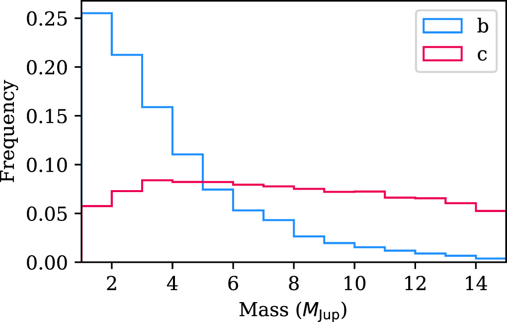
Figure 9. Injection losses γ as a function of the misalignment (Δα) of the fiber.
Download figure:
Standard image High-resolution image
Appendix B: Literature Data
We listed the photometry from the literature for PDS 70 b and PDS 70 c in Table 7. For each photometric data point, we listed the wavelength (λ) and half width (Δλ) to represent the wavelength coverage of that filter. We did not list the SPHERE IFS spectra for both planets used in the SED fit.
Table 7. Literature Photometry
| Planet | λ (μm) | Δλ (μm) | Flux (W/m2/μm) | Flux Error (W/m2/μm) | Reference |
|---|---|---|---|---|---|
| b | 1.5888 | 0.0266 | 6.43 × 10⁻¹⁷ | 1.04 × 10⁻¹⁷ | Müller et al. (2018) |
| b | 1.5888 | 0.0266 | 7.92 × 10⁻¹⁷ | 1.75 × 10⁻¹⁷ | Müller et al. (2018) |
| b | 1.6671 | 0.0278 | 6.83 × 10⁻¹⁷ | 1.05 × 10⁻¹⁷ | Müller et al. (2018) |
| b | 1.6671 | 0.0278 | 7.53 × 10⁻¹⁷ | 1.14 × 10⁻¹⁷ | Müller et al. (2018) |
| b | 2.100 | 0.051 | 1.203 × 10⁻¹⁶ | 3.46 × 10⁻¹⁷ | Müller et al. (2018) |
| b | 2.100 | 0.051 | 9.16 × 10⁻¹⁷ | 0.43 × 10⁻¹⁷ | Müller et al. (2018) |
| b | 2.2510 | 0.0545 | 1.156 × 10⁻¹⁷ | 2.57 × 10⁻¹⁷ | Müller et al. (2018) |
| b | 2.2510 | 0.0545 | 9.35 × 10⁻¹⁷ | 0.42 × 10⁻¹⁷ | Müller et al. (2018) |
| b | 3.78 | 0.35 | 7.67 × 10⁻¹⁷ | 3.09 × 10⁻¹⁷ | Müller et al. (2018) |
| b | 3.80 | 0.31 | 5.95 × 10⁻¹⁷ | 2.50 × 10⁻¹⁷ | Müller et al. (2018) |
| b | 3.776 | 0.350 | 7.52 × 10⁻¹⁷ | 1.22 × 10⁻¹⁷ | Wang et al. (2020) |
| b | 4.0555 | 0.0308 | 5.35 × 10⁻¹⁷ | 1.36 × 10⁻¹⁷ | Stolker et al. (2020) |
| b | 4.7555 | 0.2961 | 6.56 × 10⁻¹⁷ | 1.63 × 10⁻¹⁷ | Stolker et al. (2020) |
| c | 2.110 | 0.051 | 3.10 × 10⁻¹⁷ | 0.52 × 10⁻¹⁷ | Mesa et al. (2019) |
| c | 2.110 | 0.051 | 3.73 × 10⁻¹⁷ | 0.40 × 10⁻¹⁷ | Mesa et al. (2019) |
| c | 2.251 | 0.055 | 2.77 × 10⁻¹⁷ | 0.53 × 10⁻¹⁷ | Mesa et al. (2019) |
| c | 2.251 | 0.055 | 3.59 × 10⁻¹⁷ | 0.49 × 10⁻¹⁷ | Mesa et al. (2019) |
| c | 3.776 | 0.350 | 3.31 × 10⁻¹⁷ | 1.31 × 10⁻¹⁷ | Wang et al. (2020) |
Download table as: ASCIITypeset image
The literature astrometry for PDS 70 b and PDS 70 c are listed in Table 8. These were used to supplement the two GRAVITY epochs for each planet.
Table 8. Literature Astrometry
| Planet | Epoch (MJD) | Separation (mas) | Sep. Error (mas) | PA (°) | PA Error (°) | Reference |
|---|---|---|---|---|---|---|
| b | 56017 | 191.9 | 21.4 | 162.2 | 3.7 | Müller et al. (2018) |
| b | 57145 | 192.3 | 4.2 | 154.5 | 1.2 | Müller et al. (2018) |
| b | 57145 | 197.2 | 4.0 | 154.9 | 1.1 | Müller et al. (2018) |
| b | 57173 | 199.5 | 6.9 | 153.4 | 1.8 | Müller et al. (2018) |
| b | 57173 | 194.5 | 6.3 | 153.5 | 1.8 | Müller et al. (2018) |
| b | 57522 | 193.2 | 8.3 | 152.2 | 2.3 | Müller et al. (2018) |
| b | 57522 | 199.2 | 7.1 | 151.5 | 1.6 | Müller et al. (2018) |
| b | 57540 | 189.6 | 26.3 | 150.6 | 7.1 | Müller et al. (2018) |
| b | 58173 | 192.1 | 7.9 | 147.0 | 2.4 | Müller et al. (2018) |
| b | 58173 | 192.2 | 8.0 | 146.8 | 2.4 | Müller et al. (2018) |
| b | 58289 | 176.8 | 25.0 | 146.8 | 8.5 | Haffert et al. (2019) |
| b | 58642 | 175.8 | 6.9 | 140.9 | 2.2 | Wang et al. (2020) |
| c | 56017 | 191.9 | 21.4 | 162.2 | 3.7 | Müller et al. (2018) |
| c | 58173 | 209.0 | 13.0 | 281.2 | 0.5 | Mesa et al. (2019) |
| c | 58289 | 235.5 | 25.0 | 277.0 | 6.5 | Haffert et al. (2019) |
| c | 58548 | 225.0 | 8.0 | 279.9 | 0.5 | Mesa et al. (2019) |
| c | 58642 | 223.4 | 8.0 | 280.4 | 2.0 | Wang et al. (2020) |
Download table as: ASCIITypeset image
Footnotes
- ∗
Based on observations collected at the European Southern Observatory under ESO programmes 0101.C-0281(B), 1103.B-0626(A), 2103.C-5018(A), and 1104.C-0651(A).
- 27
- 28
Software available on GitHub upon request.
- 29