


ABSTRACT
Through their delivery of water and organics, near-Earth objects (NEOs) played an important role in the emergence of life on our planet. However, they also pose a hazard to the Earth, as asteroid impacts could significantly affect our civilization. Potentially hazardous asteroids (PHAs) are those that, in principle, could possibly impact the Earth within the next century, producing major damage. About 1600 PHAs are currently known, from an estimated population of 4700 ± 1450. However, a comprehensive characterization of the PHA physical properties is still missing. Here we present spectroscopic observations of 14 PHAs, which we have used to derive their taxonomy, meteorite analogs, and mineralogy. Combining our results with the literature, we investigated how PHAs are distributed as a function of their dynamical and physical properties. In general, the "carbonaceous" PHAs seem to be particularly threatening, because of their high porosity (limiting the effectiveness of the main deflection techniques that could be used in space) and low inclination and minimum orbit intersection distance (MOID) with the Earth (favoring more frequent close approaches). V-type PHAs also present low MOID values, which can produce frequent close approaches (as confirmed by the recent discovery of a limited space weathering on their surfaces). We also identified those specific objects that deserve particular attention because of their extreme rotational properties, internal strength, or possible cometary nature. For PHAs and NEOs in general, we identified a possible anti-correlation between the elongation and the rotational period, in the range of Prot ≈ 5–80 hr. This would be compatible with the behavior of gravity-dominated aggregates in rotational equilibrium. For periods ≳80–90 hr, such a trend stops, possibly under the influence of the YORP effect and collisions. However, the statistics is very low, and further observational and theoretical work is required to characterize such slow rotators.
Export citation and abstract BibTeX RIS
1. INTRODUCTION
The investigation of near-Earth objects (NEOs) emerged as one of the key topics in planetary sciences, especially because these bodies had a major role in the delivery of water and complex organic molecules to the early Earth (e.g., Alexander et al. 2012; Marty 2012; Altwegg et al. 2015). Besides being of great scientific interest, NEOs also deserve our attention because they currently represent a well-founded threat to human beings and life in general on our planet. Indeed, past impacts on the Earth have already altered the evolutionary course of life (e.g., Jablonski 1994; Nichols & Johnson 2008), and there is no reason why asteroids and comets should not continue to hit the Earth at irregular and unpredictable intervals in the future (e.g., Perna et al. 2013a, and the references therein).
Among NEOs, the definition of "potentially hazardous asteroids" (PHAs) is reserved for those objects with absolute magnitudes H ≤ 22 (i.e., diameter above ∼140 m, assuming the average NEO albedo of 0.14 found by Mainzer et al. 2011a) and whose minimum orbit intersection distance (MOID) is within 0.05 au (7.5 million km) of the Earth's orbit. PHAs are large enough to survive passage through the Earth's atmosphere and cause extensive damage on impact, and have orbits which could in principle bring them to collide with our planet within the next century (indeed, the MOID change rate is ≲0.05 au/century).10
At the time of this writing, about 1600 PHAs are known, but only ∼15% of them have been investigated to infer their composition and taxonomic type. However, the physical characterization of PHAs is essential for defining successful "mitigation strategies" in case of possible impactors. In fact, a high degree of diversity in terms of composition and spectral properties is present among the NEO population, with compositions ranging from silicaceous to carbonaceous, from basaltic to metallic, implying completely different internal densities and strengths. Whatever the scenario, it is clear that the technology needed to set up a realistic mitigation strategy depends upon having knowledge of the physical properties of the impacting object. An analysis of its surface characteristics, which are connected with the internal structure, is an essential step toward developing means of deflection or destruction of the object.
In order to enhance our knowledge of the PHA population, we started a visible and near-infrared (NIR) spectroscopic campaign to constrain their surface composition, in the framework of the NEO-SURFACE survey.11 In this paper we present our first observations for 14 PHAs, then we combine our results with the literature and perform an analysis of the entire sample (261 objects in total) of taxonomically classified PHAs, searching for correlations between physical and dynamical properties.
2. OBSERVATIONS AND DATA REDUCTION
Observations were carried out at the 3.6-m Telescopio Nazionale Galileo (TNG, La Palma, Spain), the ESO 3.6-m New Technology Telescope (NTT, La Silla, Chile), and the NASA 3.0-m Infrared Telescope Facility (IRTF, Mauna Kea, USA). The observational circumstances, as well as the instrumentation used (DOLORES and EMMI for the visible wavelength range, NICS, SofI, and SpeX for the NIR), are given in Table 1. All of the observations have been performed by orienting the slit along the parallactic angle, in order to minimize the effects of atmospheric differential refraction. The nodding technique of moving the object along the slit between two different positions was used for NIR observations, as was necessary at these wavelengths for a proper background subtraction.
Table 1. Observational Circumstances
| Object | Tel.-Instrum. | Grism/Prism, Slit | Date | UTstart | texp (s) | Airmass | Solar Analog (Airmass) |
|---|---|---|---|---|---|---|---|
| (4450) Pan | TNG-DOLORES | LR-B (0.4–0.8 μm), 2'' | 2012 Dec 20 | 23:18 | 2400 | 1.05 | Hip 49580 (1.02) |
| (5011) Ptah | NTT-EMMI | #1 (0.42–0.95 μm), 5'' | 2006 Nov 16 | 02:35 | 540 | 1.71 | HD 1368 (1.16) |
| NTT-SofI | BG (0.95–1.6 μm), 2'' | 2006 Oct 08 | 03:29 | 10 × 120 | 1.14 | Hip 10178 (1.13) | |
| NTT-SofI | RG (1.6–2.5 μm), 2'' | 2006 Oct 08 | 04:09 | 16 × 120 | 1.21 | Hip 10178 (1.13) | |
| (99942) Apophis | NTT-EMMI | #1 (0.42–0.8 μm), 1'' | 2005 Jan 18 | 01:27 | 150 | 1.15 | HD 44594 (1.18) |
| (143651) 2003 QO104 | NTT-EMMI | #1 (0.42–0.8 μm), 5'' | 2006 Nov 16 | 02:51 | 3600 | 1.40 | HD 1368 (1.16) |
| TNG-NICS | Amici (0.8–2.5 μm), 2'' | 2006 Aug 18 | 04:48 | 5 × 120 | 1.56 | Hip 113631 (1.43) | |
| (153958) 2002 AM31 | TNG-DOLORES | LR-B (0.4–0.8 μm), 2'' | 2012 Dec 20 | 22:30 | 1800 | 1.22 | SA 115-271 (1.14) |
| (163899) 2003 SD220 | TNG-DOLORES | LR-B (0.4–0.8 μm), 2'' | 2012 Dec 21 | 06:41 | 300 | 1.41 | Hip 49580 (1.02) |
| (164211) 2004 JA27 | IRTF-SpeX | low-res (0.8–2.5 μm), 0 8 8 |
2004 Oct 21 | 12:17 | 42 × 120 | 1.02 | HD 28099 (1.02) |
| (214869) 2007 PA8 | TNG-DOLORES | LR-B (0.4–0.8 μm), 2'' | 2012 Dec 21 | 05:36 | 1200 | 1.35 | Hip 49580 (1.02) |
| (350751) 2002 AW | TNG-DOLORES | LR-B (0.4–0.8 μm), 2'' | 2012 Dec 21 | 00:21 | 2400 | 1.03 | Hip 49580 (1.02) |
| 1994 XD | TNG-DOLORES | LR-B (0.4–0.8 μm), 2'' | 2012 Dec 20 | 21:40 | 1800 | 1.31 | SA 115-271 (1.14) |
| 2004 RQ10 | IRTF-SpeX | low-res (0.8–2.5 μm), 08 |
2004 Sep 23 | 10:17 | 28 × 120 | 1.09 | HD 1368 (1.11) |
| 2004 TP1 | IRTF-SpeX | low-res (0.8–2.5 μm), 08 |
2004 Oct 21 | 10:20 | 19 × 120 | 1.02 | HD 28099 (1.02) |
| 2010 BB | TNG-DOLORES | LR-B (0.4–0.8 μm), 2'' | 2013 Jan 18 | 21:38 | 1800 | 1.18 | Hip 44027 (1.18) |
| 2012 VF37 | TNG-DOLORES | LR-B(0.4–0.8 μm), 2'' | 2012 Dec 20 | 20:29 | 780 | 1.04 | Hip 49580 (1.02) |
Download table as: ASCIITypeset image
Data were reduced using standard procedures (bias and background subtraction, flat field correction, one-dimensional spectra extraction, atmospheric extinction correction—see Perna et al. 2015 for more details). Wavelength calibration was generally obtained using emission lines from several lamps. Only for the NICS/Amici data, given the very low resolution, did we use a look-up table, which is available on the instrument website. The reflectivity of our targets was then obtained by dividing their visible and NIR spectra by those of solar analogs that were observed close in time and/or in airmass to the scientific frames (see Table 1).
To increase the significance of our analysis, we searched the literature for spectral ranges to be combined with our data. The NIR spectra hereafter analyzed for Pan, Apophis, 2002 AM31, 2003 SD220, 1994 XD, and 2010 BB have been taken from the MIT-UH-IRTF Joint Campaign for NEO Spectral Reconnaissance.12 Notably, our NIR spectra of Ptah, 2003 QO104, and 2004 JA27, are completely consistent with those available from the MIT-UH-IRTF Joint Campaign for NEO Spectral Reconnaissance. The NIR spectrum of 2007 PA8 has been taken from Fornasier et al. (2015). The obtained final spectra are presented in Figures 1 and 2.
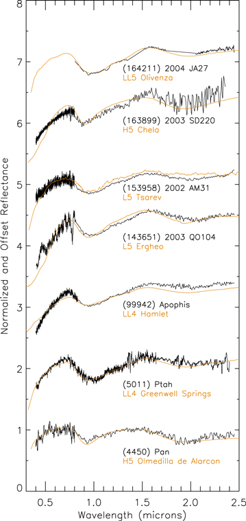
Figure 1. Reflectance spectra of Pan, Ptah, Apophis, 2003 QO104, 2002 AM31, 2003 SD220, 2004 JA27, with suggested meteorite analogs (the petrologic type is given). The spectra are normalized at 0.55 μm (if the visible wavelength range is available, otherwise at 1.25 μm) and shifted for clarity. See the text for more info.
Download figure:
Standard image High-resolution image3. TAXONOMIC CLASSIFICATION AND METEORITIC ANALOGS
We used a code based on chi-square minimization to classify our data within the taxonomic scheme by DeMeo et al. (2009). It should be noted that the different taxonomic types that are found within the NEO population give some hints about their compositions, and hence their formation region; the study of the compositional gradient of NEOs and small bodies in general, in combination with numerical simulations for investigating their dynamical mixing, allow us to retrieve information on the processes that governed the formation and the early evolution of the solar system (e.g., Walsh et al. 2011). We present the obtained results in Table 2.
Table 2. Classification Results
| Object | Albedo | Taxon | Meteorite Analog | Example Meteorite | RELAB Sample / χ2 |
|---|---|---|---|---|---|
| (4450) Pan | ... | S/Sr | H | H5 Olmedilla de Alarcon | cgn147/0.00189 |
| (5011) Ptah | 0.11a | Q | LL | LL4 Greenwell Springs | c1tb75/0.00192 |
| (99942) Apophis | 0.30b | S/Sq | LL | LL4 Hamlet | c1oc02b/0.00417 |
| (143651) 2003 QO104 | 0.14a | Sa | L | L5 Ergheo | camh21/0.00456 |
| (153958) 2002 AM31 | ... | Q | L | L5 Tsarev | c1rs65/0.00183 |
| (163899) 2003 SD220 | ... | Sr | H | H5 Chela | c1tb71/0.00670 |
| (164211) 2004 JA27 | ... | Sq/Q | LL | LL5 Olivenza | cgn139/0.00128 |
| (214869) 2007 PA8 | 0.29c | Q | L | L3 Mezo-Madaras | c1oc04c/0.00045 |
| (350751) 2002 AW | ... | B | CM | CM2 Cold Bokkeveld | cgp090/0.00220 |
| 1994 XD | ... | Q | H | H5 Barwise | cgn055/0.00149 |
| 2004 RQ10 | ... | Sq | LL | LL6 Manbhoom | mgn143/0.00098 |
| 2004 TP1 | ... | Q | LL | LL6 Jelica | cgn141/0.00100 |
| 2010 BB | ... | Q | H | H5 Nuevo Mercurio | cfmh53/0.00177 |
| 2012 VF37 | ... | Sq/Sr | LL/L/H | LL4 Soko-Banja | cgn133/0.00014 |
| L5 Knyahina | cgn077/0.00020 | ||||
| H4 Sete Lagoas | c6mh21/0.00060 |
Notes.
aThomas et al. (2011). bMüller et al. (2014). cFornasier et al. (2015).Download table as: ASCIITypeset image
The chi-square method has been also used through the M4AST13 online tool (see Popescu et al. 2012 for details on the working principles of the curve matching operated by M4AST) to compare our spectra with those of meteorites included in the RELAB database (Pieters & Hiroi 2004). This tool returns the 50 best matches over the several thousands of sample spectra in the database. Then we visually inspected 50 such proposed results to compare the asteroid and meteorite spectral parameters (band minima, spectral slopes, etc.), and we usually end up with a few meteorites belonging to the same group as the most suitable spectral analogs (Table 2). We stress that though this is the case for most of our targets, the best matches do not necessarily correspond to the lowest χ2 values: indeed, the latter are computed over the entire wavelength range, while we give more weight to a good fit of the band positions and shapes. For this reason, in this work we do not claim to have found specific "best analog meteorites," but just the "best analog meteorite groups" that overall present a better match with our asteroid spectra. For 2012 VF37, the available spectral range is not enough to discriminate between different types of ordinary chondrites (LL, L, H). As for 2002 AW, despite the fact that in this case only the visible range is available, the reflectance downturn shortward of ∼0.58 μm and the negative spectral slope longward make the association with CM carbonaceous chondrites robust. For each object in Figures 1 and 2, we plot the spectrum of a meteorite that is representative of the corresponding best analog group (the obtained χ2 is given in Table 2).
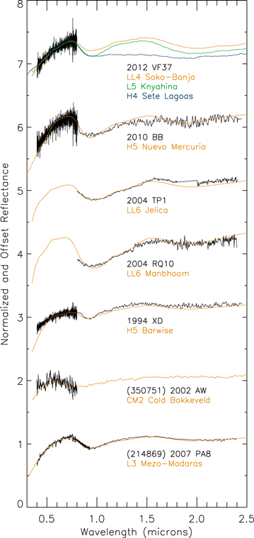
Figure 2. Reflectance spectra of 2007 PA8, 2002 AW, 1994 XD, 2004 RQ10, 2004 TP1, 2010 BB, 2012 VF37, with suggested meteorite analogs (the petrologic type is given). The spectra are normalized at 0.55 μm (if the visible wavelength range is available, otherwise at 1.25 μm) and shifted for clarity. See the text for more info.
Download figure:
Standard image High-resolution imageBoth taxonomic classification and meteorite comparisons indicate that 2002 AW is the only primitive object in our sample, whereas all of our other targets belong to the S/Q complex.
4. MINERALOGICAL ANALYSIS
To obtain more information on the surface composition of our targets, we investigated their mineralogy based on several spectral parameters (provided that the NIR range is available, see Ieva et al. 2014 for more details on our approach). We stress that the following analysis presents some limitations (see, e.g., Gaffey et al. 2002), as we are applying to asteroid spectra formulas that have been calibrated in the laboratory by measurements on minerals and meteorites. The effect of variables like the grain size, packing state, or the viewing geometry are mostly ignored, though these variables can affect the spectral slope and bands. However, our approach is the standard for the field, and the above limitations—though important—do not impede obtaining constraints, within the given errors, on the mineralogical content of the investigated asteroids.
The band minimum of the absorption at ∼1 μm (hereafter, BI) has been computed by fitting a two-degree polynomial over the bottom part of the band. Errors were computed using a Monte Carlo method, randomly sampling data 100 times and taking the standard deviation as uncertainty. The visible and NIR spectral ranges of our targets have been acquired at different epochs, preventing us from properly determining and removing the spectral continuum. Hence, to compute band centers (i.e., band minima after continuum removal), we rely on the empiric relation between band minimum and band center that has been described by Cloutis & Gafey (1991):

Then we computed BI and BII (the absorption band at ∼2 μm) areas by fitting a six-degree polynomial over each band: we considered the relative maxima of the fit at ∼0.7 and ∼1.5 μm as the extremes for BI, and between the second relative maximum and 2.5 μm as the extremes for BII. The band area ratio (hereafter, BAR) was subsequently obtained by dividing BII area by BI area. As BAR measurements are affected by temperature shifts as discussed by Sanchez et al. (2012), we applied the correction found by these authors:

To estimate the temperature T of the surface of the asteroids, we used the Standard Thermal Model by Lebofsky & Spencer (1989):

where A is the Bond albedo of the asteroid,  is the solar luminosity,
  is the infrared emissivity, η is the beaming factor, σ is the Boltzmann constant, and r is the heliocentric distance at the moment of the observations. As typical when these quantities are unknown, we assumed the geometric albedo value as an approximation of the Bond albedo, = 0.9, and η = 1 (e.g., Dunn et al. 2013). For objects with no albedo information (see Table 2), we considered the average values of their taxonomical classes (A ∼ 0.22 for S/Q-types, A ∼ 0.07 for B-types; Mainzer et al. 2011b). At this point we could infer some mineralogical properties of our targets using the following equations by Dunn et al. (2010, 2013):


where Fa is the molar content of fayalite in olivine, Fs is the molar content of ferrosilite in pyroxene, and the third expression gives the relative abundances of olivine and pyroxene in the surface minerals. The least square root means of the errors on these spectrally derived quantities are: 1.3 mol% for Fa, 1.4 mol% for Fs, and 0.03 for ol/(ol + px).
The obtained values are reported in Table 3 (where the computed spectral slope in the 0.5–0.75 μm range is also given) and shown in Figures 3 and 4 in comparison with the typical values for LL, L, and H ordinary chondrites (Dunn et al. 2010). Notably, the mineralogy of all of our targets is consistent with that of the corresponding meteoritic analog group that we identified in the previous section, making us confident about the reliability of our results.

Figure 3. Spectrally derived molar content of fayalite in targets' surface minerals, as a function of olivine/pyroxene relative abundance. The error bars (representing the least mean square error of spectrally derived mineralogies, see. Dunn et al. 2010) are the same for each of the targets, and are plotted in the lower right corner. Solid boxes represent the compositional ranges for H, L, and LL ordinary chondrites, as derived by Dunn et al. (2010).
Download figure:
Standard image High-resolution image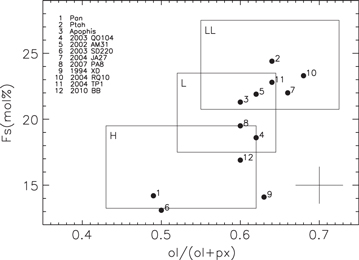
Figure 4. Spectrally derived molar content of ferrosilite in targets' surface minerals, as a function of olivine/pyroxene relative abundance. The error bars and solid boxes have the same meaning as in Figure 3.
Download figure:
Standard image High-resolution imageTable 3. Mineralogical Analysis
| Object | Slope (%/103 Å) | BIcen (μm) | BARcorr | Fa (mol%) | Fs (mol%) | ol/(ol+px) |
|---|---|---|---|---|---|---|
| (4450) Pan | 4.16 ± 0.26 | 0.925 ± 0.002 | 0.97 ± 0.05 | 15.6 ± 1.3 | 14.2 ± 1.4 | 0.49 ± 0.03 |
| (5011) Ptah | 10.05 ± 0.23 | 1.005 ± 0.001 | 0.36 ± 0.05 | 29.7 ± 1.3 | 24.4 ± 1.4 | 0.64 ± 0.03 |
| (99942) Apophis | 15.24 ± 0.24 | 0.970 ± 0.003 | 0.54 ± 0.05 | 25.5 ± 1.3 | 21.3 ± 1.4 | 0.60 ± 0.03 |
| (143651) 2003 QO104 | 21.69 ± 0.46 | 0.950 ± 0.006 | 0.43 ± 0.05 | 21.7 ± 1.3 | 18.6 ± 1.4 | 0.62 ± 0.03 |
| (153958) 2002 AM31 | 6.30 ± 0.25 | 0.975 ± 0.003 | 0.46 ± 0.05 | 26.3 ± 1.3 | 21.9 ± 1.4 | 0.62 ± 0.03 |
| (163899) 2003 SD220 | 10.90 ± 0.12 | 0.920 ± 0.003 | 0.94 ± 0.05 | 14.1 ± 1.3 | 13.1 ± 1.4 | 0.50 ± 0.03 |
| (164211) 2004 JA27 | ... | 0.976 ± 0.001 | 0.26 ± 0.05 | 26.5 ± 1.3 | 22.0 ± 1.4 | 0.66 ± 0.03 |
| (214869) 2007 PA8 | 6.72 ± 0.22 | 0.956 ± 0.001 | 0.54 ± 0.05 | 23.0 ± 1.3 | 19.5 ± 1.4 | 0.60 ± 0.03 |
| (350751) 2002 AW | −4.21 ± 1.70 | ... | ... | ... | ... | ... |
| 1994 XD | 4.16 ± 0.26 | 0.925 ± 0.002 | 0.38 ± 0.05 | 15.6 ± 1.3 | 14.1 ± 1.4 | 0.63 ± 0.03 |
| 2004 RQ10 | ... | 0.990 ± 0.003 | 0.21 ± 0.05 | 28.3 ± 1.3 | 23.3 ± 1.4 | 0.68 ± 0.03 |
| 2004 TP1 | ... | 0.984 ± 0.005 | 0.36 ± 0.05 | 27.6 ± 1.3 | 22.8 ± 1.4 | 0.64 ± 0.03 |
| 2010 BB | 9.18 ± 0.28 | 0.940 ± 0.003 | 0.52 ± 0.05 | 19.4 ± 1.3 | 16.9 ± 1.4 | 0.60 ± 0.03 |
| 2012 VF37 | 9.63 ± 0.24 | ... | ... | ... | ... | ... |
Download table as: ASCIITypeset image
5. THE PHA POPULATION: A STATISTICAL ANALYSIS
According to the population model by Mainzer et al. (2012), ∼4700 ± 1450 PHAs are expected to exist, meaning that ∼35% of them have been discovered to date. To further investigate the PHA population as a whole, and in particular to verify how the different taxonomic types are distributed with respect to other physical and dynamical properties, we combined our results with the available literature.
We started retrieving the European Asteroid Research Node (EARN)14 database of NEO physical properties, selecting those 255 PHAs with published taxonomic classifications. Of our 14 targets, 7 are classified in the present work for the first time, for a total sample of 262 targets to be considered in our analysis. The results for our remaining seven targets are in agreement with the literature. We stress that multiple taxonomic classes are listed in the EARN database for most of the objects, the main ambiguity being between the Q- and S-complex types: we discriminated between them by following DeMeo et al. (2014), who recently introduced a "flowchart" to classify asteroids belonging to the Q- or S-types. More in general (to solve ambiguities between S- and V-types, C or X, etc.), we checked the original references and gave preference to classifications based on the visible/NIR spectral range with respect to those based on visible spectra only, as well as to those considering the albedo value with respect to those which do not. In a few cases we considered a taxon other than that reported in the EARN database, when we found more recent classifications based on visible/NIR spectra (DeMeo et al. 2014; Thomas et al. 2014). As for objects classified as X-types, it is well known that they can have quite different compositions. Indeed, the X-group contains asteroids classified as either bright (albedo ≳ 0.25) "enstatitic" E-types, moderately bright (0.10 ≲ albedo ≲ 0.30) "metallic" M-types, or dark (albedo ≲ 0.1) "carbonaceous" P-types in the Tholen (1989) scheme. For this reason we reclassify as P-types those objects in the X-group with albedos lower than 10%. Object 2012 LZ1 is also assigned to the P-class as a consequence of its phase curve, which is typical for a low-albedo asteroid (Hicks et al. 2012). Finally, we removed (99248) 2001 KY66 from the following analysis, as its current classification is very uncertain (silicaceous S-type or carbonaceous T-type) and only based on low-quality visible photometry.
The final assignments of taxonomic classifications to each object are given in Table 4, together with the values of other physical and dynamical properties that will be considered in the following analysis. An overview of the taxonomic classification statistics is given by Figure 5. We note that the distribution of PHAs within the different taxa does not differentiate significantly from that of NEOs in general (e.g., Binzel et al. 2004), with the S/Q complex dominating the population as a consequence of both observational biases (albedo and phase-angle effects) and preferential transport mechanisms from the inner asteroid belt where S-type asteroids are dominant.
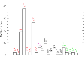
Figure 5. Distribution of PHAs within the different taxonomic classes. We redefined low-albedo X-types as P-types. The color coding is relative to the grouping scheme introduced in Section 5 (red for the "silicaceous" PHAs, magenta for the "basaltic" PHAs, black for the "carbonaceous" PHAs, green for the "miscellaneous" PHAs).
Download figure:
Standard image High-resolution imageTable 4. Physical and Dynamical Properties of PHAs
| Object | Tax. Type | H (mag) | Albedo | Rot. Period(hr) | L.C. Amplitude(mag) | a (au) | e | i (°) | q (au) | Q (au) | TJ | MOID (au) |
|---|---|---|---|---|---|---|---|---|---|---|---|---|
| 2001 FE90 | A | 20.2 | ... | ... | ... | 1.323 | 0.426 | 38.2 | 0.76 | 1.886 | 4.650 | 0.03734 |
| 2011 BT15 | A | 21.8 | ... | 0.10914 | 0.61 | 1.295 | 0.303 | 1.7 | 0.903 | 1.687 | 4.969 | 0.00108 |
| 2006 YT13 | A | 18.3 | ... | 2.433 | 0.11 | 1.935 | 0.494 | 8.8 | 0.978 | 2.891 | 3.737 | 0.01487 |
| 2004 TB18 | A | 17.7 | 0.199 | ... | ... | 1.815 | 0.451 | 13.2 | 0.997 | 2.633 | 3.894 | 0.02071 |
| 1986 PA | O | 18.4 | 0.52 | ... | ... | 1.06 | 0.444 | 11.2 | 0.589 | 1.53 | 5.703 | 0.01943 |
| 1999 CF9 | Q | 18 | ... | ... | ... | 1.078 | 0.827 | 22.8 | 0.187 | 1.97 | 5.300 | 0.03441 |
| 2000 EE14 | Q | 17.1 | ... | 2.586 | 0.26 | 1.642 | 0.886 | 10 | 0.187 | 3.097 | 3.682 | 0.00158 |
| 2001 QQ142 | Q | 18.4 | ... | ... | ... | 0.662 | 0.533 | 26.5 | 0.309 | 1.015 | 8.401 | 0.02274 |
| 2003 CR20 | Q | 18.7 | ... | ... | ... | 1.453 | 0.763 | 5.9 | 0.344 | 2.561 | 4.261 | 0.00754 |
| 1991 BN | Q | 19 | ... | ... | ... | 2.04 | 0.828 | 9.1 | 0.351 | 3.73 | 3.244 | 0.03894 |
| 1949 MA | Q | 15.9 | 0.14 | 2.273 | 0.13 | 1.182 | 0.629 | 1.5 | 0.438 | 1.926 | 5.143 | 0.00998 |
| 2000 EV70 | Q | 20.5 | ... | ... | ... | 1.621 | 0.658 | 24.4 | 0.555 | 2.687 | 3.975 | 0.02622 |
| 2003 EF54 | Q | 20 | ... | ... | ... | 1.207 | 0.531 | 1.4 | 0.566 | 1.849 | 5.127 | 0.01188 |
| 1998 HD14 | Q | 20.9 | ... | ... | ... | 2.126 | 0.729 | 5 | 0.575 | 3.676 | 3.319 | 0.00086 |
| 1998 SJ70 | Q | 18.3 | ... | 19.15 | 0.9 | 0.82 | 0.277 | 10 | 0.593 | 1.048 | 7.097 | 0.01185 |
| 1998 WZ1 | Q | 19.9 | ... | ... | ... | 2.049 | 0.709 | 5.9 | 0.596 | 3.502 | 3.420 | 0.00095 |
| 2001 QC34 | Q | 20.1 | ... | ... | ... | 0.853 | 0.286 | 4.7 | 0.609 | 1.098 | 6.874 | 0.04619 |
| 2002 NY40 | Q | 19.2 | 0.34 | 19.982 | 1.3 | 2.346 | 0.734 | 4.3 | 0.624 | 4.069 | 3.127 | 0.02028 |
| 2003 UV11 | Q | 19.5 | 0.376 | ... | ... | 1.389 | 0.541 | 25.8 | 0.638 | 2.14 | 4.528 | 0.01309 |
| 2004 TP1 | Q | 20.7 | ... | ... | ... | 1.47 | 0.560 | 6.4 | 0.647 | 2.294 | 4.415 | 0.02565 |
| 2007 RU17 | Q | 18.1 | ... | ... | ... | 2.239 | 0.705 | 7.3 | 0.661 | 3.817 | 3.247 | 0.02705 |
| 2008 HS3 | Q | 21.7 | ... | ... | ... | 0.963 | 0.313 | 7.8 | 0.662 | 1.265 | 6.213 | 0.03393 |
| 2009 WZ104 | Q | 20.5 | 0.314 | 19.304 | 0.52 | 0.855 | 0.193 | 9.8 | 0.691 | 1.02 | 6.870 | 0.03116 |
| 2010 BB | Q | 20.4 | ... | ... | ... | 1.773 | 0.6 | 5.5 | 0.709 | 2.837 | 3.864 | 0.01915 |
| 2011 PS | Q | 20.4 | ... | ... | ... | 2.565 | 0.721 | 5 | 0.715 | 4.415 | 2.998 | 0.02778 |
| 2004 NL8 | Q | 17.1 | ... | ... | ... | 1.982 | 0.634 | 6.7 | 0.725 | 3.24 | 3.573 | 0.02854 |
| 2007 PA8 | Q | 16.2 | ... | 95.1 | 0.7 | 1.29 | 0.389 | 7.5 | 0.788 | 1.792 | 4.943 | 0.0282 |
| 1998 DV9 | Q | 18.2 | ... | ... | ... | 1.636 | 0.5 | 7.4 | 0.818 | 2.454 | 4.143 | 0.02497 |
| 2003 FH | Q | 19 | ... | ... | ... | 1.21 | 0.323 | 2.7 | 0.819 | 1.6 | 5.212 | 0.01388 |
| 1982 HR | Q | 19 | 0.357 | 3.51 | 0.25 | 1.609 | 0.473 | 3 | 0.849 | 2.37 | 4.212 | 0.0419 |
| 2000 EA14 | Q | 21.1 | ... | ... | ... | 1.444 | 0.398 | 3.4 | 0.869 | 2.019 | 4.568 | 0.02068 |
| 2002 NV16 | Q | 21.4 | ... | 0.90672 | 0.4 | 1.806 | 0.515 | 3.7 | 0.876 | 2.736 | 3.889 | 0.02656 |
| 1959 LM | Q | 14.4 | 0.097 | 3.5595 | 0.64 | 1.117 | 0.202 | 3.6 | 0.891 | 1.343 | 5.564 | 0.04336 |
| 2000 AC6 | Q | 21.5 | 0.143 | ... | ... | 1.842 | 0.507 | 5.4 | 0.909 | 2.775 | 3.846 | 0.04784 |
| 2005 ED318 | Q | 20.8 | 0.212 | 17.157 | 0.22 | 1.128 | 0.188 | 6.2 | 0.917 | 1.34 | 5.522 | 0.02827 |
| 1990 MU | Q | 15.1 | 0.52 | 14.218 | 0.68 | 1.703 | 0.452 | 4.6 | 0.934 | 2.473 | 4.073 | 0.03177 |
| 6743 P-L | Q | 16.4 | 0.11 | ... | ... | 2.824 | 0.662 | 2 | 0.956 | 4.692 | 2.946 | 0.02434 |
| 1991 VK | Q | 16.9 | ... | 4.2096 | 0.49 | 2.164 | 0.555 | 4.3 | 0.962 | 3.365 | 3.474 | 0.02379 |
| 2001 FM129 | Q | 17.6 | 0.252 | ... | ... | 1.237 | 0.22 | 3.5 | 0.965 | 1.509 | 5.156 | 0.02773 |
| 2002 LY45 | Q | 17 | ... | ... | ... | 1.423 | 0.311 | 9.3 | 0.98 | 1.865 | 4.637 | 0.01236 |
| 2002 AM31 | Q | 18.3 | ... | ... | ... | 1.744 | 0.433 | 8.7 | 0.988 | 2.5 | 4.015 | 0.00352 |
| 1932 HA | Q | 16.4 | 0.26 | 3.065 | 0.38 | 1.85 | 0.449 | 2.4 | 1.019 | 2.681 | 3.877 | 0.00933 |
| 1994 XD | Q | 19.1 | ... | 2.7365 | 0.08 | 1.351 | 0.226 | 8.2 | 1.046 | 1.656 | 4.834 | 0.03633 |
| 1992 SK | S | 17.4 | 0.28 | 7.3198 | 0.75 | 1.467 | 0.926 | 28 | 0.109 | 2.826 | 3.901 | 0.03429 |
| 1999 XA143 | S | 17 | 0.175 | 9.849 | 0.49 | 0.642 | 0.688 | 38.9 | 0.2 | 1.084 | 8.502 | 0.0132 |
| 1989 UR | S | 18.5 | 0.13 | 73 | 0.5 | 1.341 | 0.796 | 31.5 | 0.274 | 2.407 | 4.404 | 0.028 |
| 1998 OH | S | 15.8 | 0.232 | 5.833 | 0.12 | 1.701 | 0.826 | 38.9 | 0.295 | 3.107 | 3.560 | 0.0043 |
| 1999 GK4 | S | 15.9 | 0.176 | 3.891 | 0.18 | 0.859 | 0.643 | 19.2 | 0.307 | 1.41 | 6.645 | 0.04599 |
| 1997 BR | S | 18 | ... | 33.644 | 1.2 | 2.704 | 0.859 | 48.4 | 0.382 | 5.026 | 2.414 | 0.04145 |
| 1997 BQ | S | 18.1 | ... | ... | ... | 0.937 | 0.57 | 14.3 | 0.403 | 1.471 | 6.229 | 0.00546 |
| 1999 TF211 | S | 15.2 | ... | ... | ... | 0.718 | 0.418 | 7.3 | 0.418 | 1.019 | 7.917 | 0.01056 |
| 2000 HA24 | S | 19.1 | ... | ... | ... | 0.747 | 0.36 | 8.6 | 0.478 | 1.016 | 7.665 | 0.02226 |
| 2002 CQ11 | S | 20 | 0.34 | 2.6 | 0.2 | 2.434 | 0.795 | 2 | 0.5 | 4.367 | 2.967 | 0.0042 |
| 1998 FW4 | S | 19.7 | ... | 17.38 | 0.34 | 0.823 | 0.369 | 17.5 | 0.519 | 1.127 | 7.028 | 0.04198 |
| 2000 GJ147 | S | 19.4 | 0.109 | ... | ... | 1.704 | 0.689 | 8.7 | 0.529 | 2.88 | 3.873 | 0.00297 |
| 2000 JG5 | S | 18.5 | ... | 6.051 | 0.91 | 0.978 | 0.428 | 2.5 | 0.559 | 1.397 | 6.103 | 0.01932 |
| 2002 SY50 | S | 17.6 | ... | 4.823 | 0.52 | 1.442 | 0.586 | 5.5 | 0.596 | 2.288 | 4.458 | 0.02858 |
| 1978 CA | S | 17.1 | 0.199 | 3.7538 | 0.8 | 1.552 | 0.615 | 25 | 0.597 | 2.506 | 4.133 | 0.01308 |
| 1951 RA | S | 16.5 | 0.19 | 5.2233 | 1.55 | 1.026 | 0.375 | 6.8 | 0.642 | 1.41 | 5.889 | 0.014 |
| 2001 JM1 | S | 19.1 | ... | 5.7516 | 0.15 | 1.416 | 0.547 | 33.7 | 0.642 | 2.19 | 4.401 | 0.02603 |
| 2000 MU1 | S | 19.9 | ... | ... | ... | 1.057 | 0.344 | 25.2 | 0.693 | 1.42 | 5.689 | 0.006 |
| 1998 VO | S | 20.4 | 0.28 | ... | ... | 1.924 | 0.639 | 10.8 | 0.693 | 3.154 | 3.623 | 0.00283 |
| 1997 QK1 | S | 20.3 | ... | ... | ... | 1.08 | 0.356 | 10.3 | 0.696 | 1.464 | 5.656 | 0.03451 |
| 1998 WB2 | S | 21.8 | 0.151 | 0.313 | 0.6 | 2.511 | 0.722 | 3.5 | 0.699 | 4.324 | 3.031 | 0.00763 |
| 1999 FA | S | 20.7 | ... | 10.092 | 1.2 | 0.934 | 0.236 | 6.5 | 0.714 | 1.154 | 6.389 | 0.00597 |
| 2000 TU28 | S | 20.8 | ... | ... | ... | 1.76 | 0.579 | 7.1 | 0.741 | 2.779 | 3.897 | 0.02428 |
| 2000 YF29 | S | 20.3 | 0.27 | ... | ... | 2.199 | 0.663 | 3 | 0.741 | 3.657 | 3.338 | 0.04624 |
| 2002 AV | S | 20.9 | ... | ... | ... | 1.443 | 0.484 | 4.1 | 0.744 | 2.141 | 4.525 | 0.00071 |
| 2002 QH10 | S | 20.3 | ... | ... | ... | 0.922 | 0.191 | 3.3 | 0.746 | 1.098 | 6.469 | 0.00025 |
| 2003 ED50 | S | 20.8 | ... | ... | ... | 1.917 | 0.609 | 5.8 | 0.749 | 3.084 | 3.672 | 0.03383 |
| 2005 GU | S | 20 | ... | ... | ... | 1.844 | 0.582 | 38.5 | 0.771 | 2.916 | 3.579 | 0.04176 |
| 2006 UL217 | S | 20.8 | ... | ... | ... | 1.14 | 0.319 | 2.2 | 0.776 | 1.503 | 5.451 | 0.02731 |
| 2001 XN254 | S | 17.6 | ... | ... | ... | 1.642 | 0.526 | 0.9 | 0.778 | 2.506 | 4.124 | 0.01214 |
| 2008 DE | S | 19.5 | ... | ... | ... | 1.983 | 0.591 | 9.6 | 0.812 | 3.154 | 3.606 | 0.01773 |
| 2008 EE5 | S | 19.7 | ... | ... | ... | 1.382 | 0.411 | 8.9 | 0.815 | 1.95 | 4.693 | 0.00245 |
| 2008 QS11 | S | 19.9 | 0.08 | 46.65 | 0.3 | 1.976 | 0.587 | 2.4 | 0.816 | 3.135 | 3.630 | 0.01474 |
| 2009 OG | S | 16.2 | ... | ... | ... | 1.245 | 0.335 | 13.3 | 0.828 | 1.663 | 5.076 | 0.03042 |
| 2009 UN3 | S | 18.6 | ... | 4.123 | 0.5 | 1.075 | 0.227 | 10.1 | 0.831 | 1.318 | 5.712 | 0.02668 |
| 2011 LJ19 | S | 21.4 | ... | ... | ... | 1.298 | 0.356 | 4.1 | 0.835 | 1.76 | 4.940 | 0.02149 |
| 2011 WV134 | S | 17.1 | ... | 10.105 | 0.23 | 1.341 | 0.378 | 9.6 | 0.835 | 1.847 | 4.807 | 0.01131 |
| 2011 XA3 | S | 20.5 | ... | 0.73 | 0.8 | 2.465 | 0.661 | 2.8 | 0.836 | 4.094 | 3.142 | 0.01896 |
| 2012 QG42 | S | 20.9 | ... | 24.22 | 1.18 | 2.243 | 0.626 | 9.8 | 0.839 | 3.646 | 3.329 | 0.02275 |
| 1999 AQ10 | S | 20.4 | ... | 2.79 | 0.2 | 1.248 | 0.325 | 15.3 | 0.843 | 1.654 | 5.063 | 0.04585 |
| 1998 WT | S | 17.7 | 0.27 | 10.24 | 0.11 | 1.133 | 0.252 | 17.7 | 0.847 | 1.418 | 5.453 | 0.00816 |
| 2001 BE10 | S | 19.1 | 0.253 | 4.196 | 0.32 | 1.373 | 0.383 | 13.1 | 0.848 | 1.898 | 4.714 | 0.01047 |
| 2001 FO32 | S | 17.7 | ... | ... | ... | 1.285 | 0.33 | 34.5 | 0.861 | 1.708 | 4.822 | 0.04247 |
| 2004 QT24 | S | 18.3 | 0.42 | ... | ... | 0.945 | 0.072 | 44.8 | 0.877 | 1.012 | 6.110 | 0.02129 |
| 2000 AZ93 | S | 21 | 0.037 | ... | ... | 1.073 | 0.183 | 15.6 | 0.877 | 1.269 | 5.709 | 0.00005 |
| 2003 FC5 | S | 18.6 | ... | 129.5 | 0.5 | 1.508 | 0.417 | 16.7 | 0.88 | 2.136 | 4.388 | 0.03752 |
| 1996 SK | S | 16.7 | ... | 4.656 | 0.45 | 1.123 | 0.214 | 26.1 | 0.883 | 1.363 | 5.449 | 0.01562 |
| 1990 UA | S | 19.7 | ... | ... | ... | 1.162 | 0.237 | 25 | 0.887 | 1.437 | 5.310 | 0.0256 |
| 2008 AF4 | S | 19.7 | ... | ... | ... | 2.784 | 0.679 | 6 | 0.893 | 4.674 | 2.937 | 0.02419 |
| 1998 QC1 | S | 19.7 | ... | ... | ... | 1.346 | 0.328 | 33.5 | 0.904 | 1.788 | 4.667 | 0.00018 |
| 1997 XF11 | S | 16.8 | ... | 3.2573 | 0.82 | 1.746 | 0.478 | 11 | 0.91 | 2.581 | 3.979 | 0.03606 |
| 1999 YG3 | S | 19.1 | ... | ... | ... | 2.412 | 0.622 | 2.4 | 0.912 | 3.912 | 3.222 | 0.01608 |
| 2009 AV | S | 18.1 | 0.146 | ... | ... | 2.314 | 0.605 | 29.5 | 0.914 | 3.715 | 3.173 | 0.00796 |
| 1982 XB | S | 18.9 | 0.34 | 9.0046 | 0.2 | 1.541 | 0.406 | 24.5 | 0.916 | 2.167 | 4.282 | 0.02884 |
| 2002 LV | S | 16.6 | 0.15 | 6.195 | 0.94 | 1.335 | 0.306 | 17.2 | 0.927 | 1.743 | 4.819 | 0.01412 |
| 2000 GF2 | S | 20.5 | ... | ... | ... | 1.43 | 0.349 | 9.9 | 0.931 | 1.929 | 4.607 | 0.022 |
| 2005 UL5 | S | 20.2 | ... | ... | ... | 1.078 | 0.133 | 12 | 0.935 | 1.221 | 5.709 | 0.00649 |
| 1987 SY | S | 17.1 | ... | 56.48 | 0.64 | 1.123 | 0.165 | 37.1 | 0.938 | 1.308 | 5.364 | 0.0229 |
| 1987 SB | S | 15.6 | 0.297 | 100 | 1 | 1.491 | 0.371 | 6.3 | 0.938 | 2.045 | 4.478 | 0.00939 |
| 1998 ML14 | S | 16.9 | 0.27 | 14.28 | 0.15 | 2.014 | 0.534 | 8.2 | 0.938 | 3.091 | 3.625 | 0.04321 |
| 2000 ED104 | S | 17.3 | 0.18 | 43 | 1.1 | 2.387 | 0.605 | 23.7 | 0.942 | 3.832 | 3.167 | 0.01034 |
| 2001 KZ66 | S | 16.8 | ... | ... | ... | 1.03 | 0.074 | 45.9 | 0.954 | 1.106 | 5.669 | 0.0205 |
| 2002 QF15 | S | 16.4 | ... | ... | ... | 2.448 | 0.61 | 39.2 | 0.954 | 3.942 | 2.968 | 0.02006 |
| 1994 PC1 | S | 16.8 | 0.19 | 2.5999 | 0.29 | 1.861 | 0.482 | 12.5 | 0.963 | 2.758 | 3.819 | 0.0079 |
| 1991 CS | S | 17.4 | 0.1 | 2.3893 | 0.29 | 2.784 | 0.647 | 2.9 | 0.984 | 4.583 | 2.983 | 0.01701 |
| 1998 FG2 | S | 21.6 | ... | ... | ... | 2.327 | 0.576 | 37.4 | 0.986 | 3.667 | 3.104 | 0.02422 |
| 1998 SS49 | S | 15.7 | 0.076 | 5.37 | 0.18 | 2.044 | 0.517 | 12.7 | 0.987 | 3.102 | 3.592 | 0.00707 |
| 1999 NC43 | S | 16 | 0.14 | 34.1 | 0.93 | 2.621 | 0.621 | 1.5 | 0.993 | 4.248 | 3.097 | 0.00515 |
| 2000 SY2 | S | 16 | 0.23 | 8.8 | 0.1 | 1.962 | 0.492 | 5.3 | 0.997 | 2.927 | 3.716 | 0.02164 |
| 2002 CE | S | 15 | 0.31 | 2.6149 | 0.09 | 1.371 | 0.269 | 40.8 | 1.002 | 1.739 | 4.544 | 0.04911 |
| 1991 EE | S | 17 | 0.3 | 3.045 | 0.14 | 1.715 | 0.414 | 14.8 | 1.006 | 2.425 | 4.044 | 0.00565 |
| 2004 MN4 | S | 19.1 | 0.3 | 30.56 | 1 | 1.461 | 0.311 | 17.1 | 1.007 | 1.915 | 4.524 | 0.04632 |
| 1998 CS1 | S | 17.6 | ... | 2.765 | 0.2 | 1.835 | 0.446 | 3.9 | 1.017 | 2.652 | 3.896 | 0.03811 |
| 2003 QO104 | S | 16 | 0.14 | 114.09 | 1.6 | 2.077 | 0.508 | 43.7 | 1.023 | 3.131 | 3.292 | 0.02758 |
| 2000 RS11 | S | 19.1 | 0.35 | 4.444 | 1.31 | 2.325 | 0.558 | 1.9 | 1.027 | 3.622 | 3.347 | 0.04491 |
| 1994 CC | S | 17.7 | ... | 2.39 | 0.09 | 2.361 | 0.561 | 4.8 | 1.037 | 3.685 | 3.315 | 0.04864 |
| 1994 AW1 | Sa | 17.4 | ... | 2.5193 | 0.12 | 1.491 | 0.578 | 7.8 | 0.629 | 2.354 | 4.355 | 0.01943 |
| 2007 SJ | Sa | 17.2 | ... | 2.718 | 0.17 | 1.28 | 0.321 | 17.1 | 0.87 | 1.691 | 4.963 | 0.0083 |
| 2006 VV2 | Sa | 16.8 | ... | 2.425 | 0.42 | 1.638 | 0.417 | 4.7 | 0.955 | 2.321 | 4.193 | 0.016 |
| 2005 NB7 | Sa | 18.7 | ... | 3.4883 | 0.13 | 2.136 | 0.524 | 11.6 | 1.016 | 3.255 | 3.505 | 0.005 |
| 1999 KW4 | Sa | 16.5 | ... | 2.765 | 0.12 | 1.105 | 0.076 | 24.1 | 1.021 | 1.188 | 5.548 | 0.01953 |
| 1999 YD | Sk | 21.1 | ... | ... | ... | 2.298 | 0.748 | 11.9 | 0.58 | 4.017 | 3.127 | 0.04579 |
| 2002 BK25 | Sk | 18.3 | ... | ... | ... | 1.01 | 0.237 | 9.8 | 0.77 | 1.25 | 5.995 | 0.00392 |
| 2005 WK4 | Sk | 20.1 | ... | 2.595 | 0.36 | 2.464 | 0.593 | 1.4 | 1.003 | 3.924 | 3.219 | 0.02755 |
| 2004 VG64 | Sq | 18.3 | ... | ... | ... | 0.674 | 0.665 | 2 | 0.225 | 1.122 | 8.258 | 0.00552 |
| 2002 UQ3 | Sq | 17.6 | ... | ... | ... | 0.762 | 0.602 | 20.3 | 0.303 | 1.22 | 7.402 | 0.00358 |
| 2001 UA5 | Sq | 17.5 | ... | ... | ... | 2.202 | 0.858 | 17.6 | 0.313 | 4.092 | 3.000 | 0.01454 |
| 2002 FB3 | Sq | 16.4 | 0.18 | ... | ... | 0.968 | 0.655 | 36.3 | 0.334 | 1.603 | 5.901 | 0.02867 |
| 2002 OD20 | Sq | 18.8 | ... | 2.4201 | 0.11 | 1.323 | 0.702 | 20.9 | 0.395 | 2.252 | 4.604 | 0.02376 |
| 2004 JA27 | Sq | 19.4 | ... | ... | ... | 1.897 | 0.767 | 13.8 | 0.442 | 3.351 | 3.495 | 0.03414 |
| 2005 GN59 | Sq | 17.4 | ... | 38.62 | 1.4 | 0.844 | 0.45 | 5.9 | 0.464 | 1.224 | 6.881 | 0.0071 |
| 1998 QS52 | Sq | 14.3 | ... | 2.9 | 0.24 | 2.222 | 0.776 | 3.1 | 0.497 | 3.947 | 3.165 | 0.01666 |
| 1998 BB10 | Sq | 20.3 | ... | ... | ... | 0.863 | 0.423 | 3.3 | 0.498 | 1.229 | 6.766 | 0.02326 |
| 2004 VW14 | Sq | 19.4 | ... | 2.5009 | 0.14 | 1.271 | 0.585 | 5.1 | 0.527 | 2.015 | 4.892 | 0.00543 |
| 1999 JE1 | Sq | 19.9 | ... | ... | ... | 2.576 | 0.773 | 0.6 | 0.585 | 4.567 | 2.912 | 0.00265 |
| 1999 MN | Sq | 20.5 | ... | 5.494 | 0.65 | 1.1 | 0.446 | 16.7 | 0.609 | 1.59 | 5.519 | 0.00912 |
| 2000 QW7 | Sq | 19.8 | ... | 71.3 | 1 | 1.655 | 0.624 | 6.1 | 0.622 | 2.688 | 4.020 | 0.00438 |
| 2001 EC | Sq | 18.6 | ... | ... | ... | 2.175 | 0.713 | 2.5 | 0.624 | 3.725 | 3.298 | 0.00314 |
| 2001 JV1 | Sq | 21.4 | ... | ... | ... | 1.152 | 0.413 | 3.9 | 0.676 | 1.627 | 5.372 | 0.02641 |
| 2001 TC45 | Sq | 19.2 | ... | ... | ... | 2.192 | 0.668 | 8.9 | 0.729 | 3.656 | 3.328 | 0.00192 |
| 2001 XU30 | Sq | 19.8 | ... | ... | ... | 1.272 | 0.425 | 11.5 | 0.732 | 1.812 | 4.968 | 0.02317 |
| 2002 GO5 | Sq | 17.9 | 0.24 | ... | ... | 1.72 | 0.562 | 28.8 | 0.754 | 2.685 | 3.858 | 0.03921 |
| 2002 VP69 | Sq | 17.9 | ... | ... | ... | 1.847 | 0.589 | 51.3 | 0.758 | 2.936 | 3.419 | 0.01406 |
| 2004 RQ10 | Sq | 20.9 | ... | 5.76 | 0.68 | 2.218 | 0.642 | 15.6 | 0.794 | 3.643 | 3.310 | 0.02151 |
| 2006 HQ30 | Sq | 21.2 | ... | ... | ... | 1.565 | 0.477 | 7 | 0.819 | 2.31 | 4.282 | 0.00321 |
| 2008 UE7 | Sq | 20.4 | ... | 3.25146 | 0.25 | 2.118 | 0.601 | 3.9 | 0.846 | 3.391 | 3.474 | 0.00987 |
| 2009 SQ104 | Sq | 21 | ... | 6.8532 | 1.5 | 1.234 | 0.311 | 12.8 | 0.85 | 1.618 | 5.119 | 0.00139 |
| 2012 VF37 | Sq | 21 | ... | ... | ... | 1.365 | 0.377 | 8.7 | 0.851 | 1.88 | 4.750 | 0.01506 |
| 2013 RH74 | Sq | 20.3 | ... | 5.346 | 0.36 | 2.459 | 0.654 | 4.9 | 0.852 | 4.067 | 3.152 | 0.01442 |
| 1998 VD35 | Sq | 20.4 | ... | ... | ... | 1.366 | 0.369 | 4.2 | 0.862 | 1.87 | 4.759 | 0.02638 |
| 1991 JW | Sq | 19.5 | 0.161 | 3.15 | 0.17 | 2.69 | 0.676 | 5.4 | 0.871 | 4.51 | 2.989 | 0.02704 |
| 1947 XC | Sq | 16.9 | 0.24 | 26 | 0.1 | 1.145 | 0.238 | 8.7 | 0.873 | 1.418 | 5.445 | 0.00732 |
| 2000 PN9 | Sq | 16.1 | ... | 2.5325 | 0.15 | 1.657 | 0.468 | 6.6 | 0.882 | 2.431 | 4.131 | 0.04939 |
| 1976 UA | Sq | 20.2 | 0.6 | 3.358 | 0.11 | 1.235 | 0.28 | 19 | 0.889 | 1.58 | 5.098 | 0.03634 |
| 1998 SF36 | Sq | 19.5 | 0.36 | 12.132 | 0.85 | 1.319 | 0.326 | 18 | 0.889 | 1.75 | 4.850 | 0.02353 |
| 2000 CH59 | Sq | 19.8 | ... | ... | ... | 1.344 | 0.335 | 7 | 0.894 | 1.794 | 4.822 | 0.01533 |
| 1981 ET3 | Sq | 14.5 | 0.146 | 2.3581 | 0.18 | 2.137 | 0.577 | 9.5 | 0.903 | 3.371 | 3.467 | 0.00015 |
| 1999 JT6 | Sq | 16 | ... | 5.806 | 0.14 | 1.648 | 0.448 | 4 | 0.91 | 2.387 | 4.161 | 0.00915 |
| 2003 KU2 | Sq | 17.6 | ... | 3.278 | 0.2 | 1.039 | 0.119 | 8.7 | 0.916 | 1.162 | 5.885 | 0.01946 |
| 2002 DU3 | Sq | 20.7 | ... | ... | ... | 1.285 | 0.28 | 4 | 0.926 | 1.645 | 5.001 | 0.03823 |
| 2006 VQ13 | Sq | 20 | ... | ... | ... | 2.284 | 0.594 | 5.5 | 0.927 | 3.642 | 3.339 | 0.01835 |
| 1993 DQ1 | Sq | 16.5 | ... | 9.58 | 0.2 | 2.206 | 0.575 | 5.5 | 0.936 | 3.475 | 3.419 | 0.01247 |
| 1989 AC | Sq | 15.3 | 0.13 | 176 | 1.2 | 2.534 | 0.629 | 0.4 | 0.939 | 4.129 | 3.138 | 0.00608 |
| 1993 EA | Sq | 16.9 | ... | 2.497 | 0.1 | 2.018 | 0.529 | 10.2 | 0.952 | 3.085 | 3.618 | 0.02676 |
| 1989 QF | Sq | 18.7 | 0.57 | 3.5558 | 0.08 | 1.324 | 0.28 | 1.6 | 0.953 | 1.695 | 4.898 | 0.01297 |
| 1991 JX | Sq | 19.1 | ... | 6.0264 | 0.64 | 1.853 | 0.483 | 9.1 | 0.957 | 2.749 | 3.840 | 0.02286 |
| 2001 CV26 | Sq | 16.4 | 0.29 | 2.429 | 0.16 | 1.666 | 0.424 | 2.3 | 0.96 | 2.371 | 4.147 | 0.03256 |
| 1991 AQ | Sq | 17.2 | ... | ... | ... | 1.704 | 0.436 | 6.6 | 0.962 | 2.447 | 4.077 | 0.02246 |
| 1993 KH | Sq | 18.6 | ... | ... | ... | 2.486 | 0.612 | 2.3 | 0.963 | 4.008 | 3.185 | 0.02493 |
| 2000 GK137 | Sq | 17.4 | ... | 4.03 | 0.17 | 1.137 | 0.144 | 13.9 | 0.973 | 1.302 | 5.474 | 0.02568 |
| 2003 YE45 | Sq | 17.6 | 0.05 | ... | ... | 1.995 | 0.507 | 10.1 | 0.984 | 3.006 | 3.659 | 0.01598 |
| 2002 GT | Sq | 18.7 | ... | 3.7663 | 0.36 | 1.787 | 0.445 | 9.9 | 0.991 | 2.583 | 3.946 | 0.03254 |
| 2000 DP107 | Sq | 18 | ... | 2.7745 | 0.18 | 1.768 | 0.423 | 22.2 | 1.021 | 2.516 | 3.921 | 0.04488 |
| 2007 DT103 | Sq | 20 | ... | 2.703 | 0.09 | 2.597 | 0.606 | 12 | 1.022 | 4.171 | 3.103 | 0.00592 |
| 1991 VH | Sq | 17 | 0.26 | 2.6236 | 0.08 | 2.036 | 0.493 | 10 | 1.033 | 3.04 | 3.627 | 0.02749 |
| 1937 UB | Sq | 17.6 | ... | 13.894 | 0.06 | 1.947 | 0.468 | 4.2 | 1.036 | 2.858 | 3.751 | 0.03081 |
| 1999 DJ4 | Sq | 18.6 | 0.3 | 2.5141 | 0.11 | 1.865 | 0.442 | 5.7 | 1.04 | 2.689 | 3.859 | 0.03225 |
| 2000 OJ8 | Sr | 16.7 | ... | ... | ... | 1.895 | 0.811 | 20.4 | 0.359 | 3.432 | 3.407 | 0.00076 |
| 2003 SD220 | Sr | 16.9 | ... | ... | ... | 0.828 | 0.21 | 8.5 | 0.654 | 1.002 | 7.056 | 0.01765 |
| 2004 VC | Sr | 18.7 | 0.042 | ... | ... | 1.29 | 0.299 | 64 | 0.904 | 1.676 | 4.450 | 0.04398 |
| 1975 YA | Sr | 16 | 0.214 | 2.391 | 0.08 | 2.36 | 0.565 | 6.2 | 1.026 | 3.694 | 3.309 | 0.03678 |
| 1998 WZ6 | V | 17.3 | ... | ... | ... | 0.811 | 0.467 | 10.3 | 0.433 | 1.19 | 7.103 | 0.01869 |
| 1973 EA | V | 15.6 | ... | 5.22 | 0.73 | 1.588 | 0.724 | 3.1 | 0.438 | 2.738 | 4.038 | 0.02107 |
| 1996 JA1 | V | 21 | 0.3 | 5.227 | 0.8 | 1.43 | 0.682 | 3.5 | 0.455 | 2.405 | 4.404 | 0.01355 |
| 1997 GL3 | V | 19.1 | ... | 7.572 | 0.28 | 2.276 | 0.781 | 6.7 | 0.499 | 4.053 | 3.106 | 0.00146 |
| 2000 DO1 | V | 20.3 | ... | ... | ... | 0.929 | 0.406 | 4.7 | 0.552 | 1.306 | 6.371 | 0.03342 |
| 2000 SP43 | V | 18.6 | ... | ... | ... | 1.776 | 0.65 | 39.8 | 0.622 | 2.931 | 3.612 | 0.00399 |
| 1992 FE | V | 17.1 | 0.53 | 5.68175 | 0.2 | 2.564 | 0.701 | 21.6 | 0.767 | 4.361 | 2.960 | 0.01369 |
| 2001 XR31 | V | 16.5 | ... | ... | ... | 1.11 | 0.292 | 44.1 | 0.786 | 1.434 | 5.322 | 0.00307 |
| 1996 EN | V | 16.3 | 0.217 | ... | ... | 1.506 | 0.431 | 38 | 0.858 | 2.155 | 4.220 | 0.0215 |
| 2003 YT1 | V | 16.2 | 0.48 | 2.343 | 0.18 | 1.452 | 0.408 | 24.8 | 0.86 | 2.045 | 4.459 | 0.03503 |
| 2008 BT18 | V | 18.3 | ... | 2.726 | 0.04 | 2.222 | 0.593 | 8.1 | 0.904 | 3.54 | 3.383 | 0.01021 |
| 2004 FG11 | V | 21 | 0.306 | ... | ... | 1.707 | 0.437 | 22.7 | 0.961 | 2.452 | 3.999 | 0.02542 |
| 1999 RQ36 | B | 20.2 | 0.046 | 4.2905 | 0.17 | 1.271 | 0.89 | 22.2 | 0.14 | 2.402 | 4.511 | 0.0196 |
| 1997 NC1 | B | 18 | ... | ... | ... | 0.938 | 0.321 | 5.4 | 0.637 | 1.24 | 6.348 | 0.01016 |
| 2000 EW70 | B | 21.3 | 0.045 | ... | ... | 0.866 | 0.208 | 16.7 | 0.685 | 1.046 | 6.773 | 0.01729 |
| 1983 TB | B | 13.9 | 0.11 | 3.6032 | 0.26 | 1.468 | 0.482 | 3.1 | 0.76 | 2.175 | 4.474 | 0.00674 |
| 2002 AW | B | 20.8 | ... | ... | ... | 1.071 | 0.256 | 0.6 | 0.796 | 1.345 | 5.736 | 0.00474 |
| 2001 PM9 | B | 18.8 | 0.018 | ... | ... | 1.126 | 0.204 | 6 | 0.897 | 1.355 | 5.527 | 0.00252 |
| 1988 XB | B | 18.6 | ... | ... | ... | 1.618 | 0.416 | 8.1 | 0.946 | 2.291 | 4.220 | 0.004 |
| 1986 JK | C | 18.3 | ... | ... | ... | 1.157 | 0.431 | 0.3 | 0.659 | 1.656 | 5.348 | 0.00044 |
| 1999 JU3 | C | 19.2 | 0.07 | 7.625 | 0.2 | 0.915 | 0.265 | 1.3 | 0.673 | 1.157 | 6.495 | 0.01411 |
| 2000 RW37 | C | 19.9 | ... | ... | ... | 2.619 | 0.722 | 8.3 | 0.727 | 4.512 | 2.958 | 0.01849 |
| 2002 CU11 | C | 18.5 | 0.408 | ... | ... | 2.094 | 0.639 | 2.6 | 0.756 | 3.431 | 3.460 | 0.01016 |
| 1998 HT31 | C | 20.8 | ... | ... | ... | 2.53 | 0.696 | 6.8 | 0.768 | 4.292 | 3.051 | 0.03082 |
| 1998 QK28 | C | 19.4 | ... | ... | ... | 2 | 0.605 | 3.6 | 0.791 | 3.209 | 3.587 | 0.00254 |
| 2008 SV11 | C | 18.4 | ... | 32.4 | 0.5 | 1.903 | 0.553 | 8.3 | 0.851 | 2.955 | 3.731 | 0.02903 |
| 2009 KC3 | C | 18 | 0.023 | ... | ... | 1.22 | 0.295 | 48.8 | 0.86 | 1.58 | 4.875 | 0.00001 |
| 2006 AS2 | C | 20.4 | ... | 4.48 | 0.2 | 0.958 | 0.084 | 7.4 | 0.878 | 1.038 | 6.280 | 0.01471 |
| 1996 RG3 | C | 18.4 | ... | ... | ... | 1.839 | 0.517 | 29.5 | 0.889 | 2.789 | 3.715 | 0.04549 |
| 2005 YU55 | C | 21.2 | 0.065 | 19.31 | 0.2 | 1.248 | 0.25 | 13.7 | 0.935 | 1.56 | 5.091 | 0.00822 |
| 2008 EV5 | C | 20 | 0.13 | 3.725 | 0.05 | 1.403 | 0.329 | 13.6 | 0.942 | 1.865 | 4.662 | 0.03658 |
| 1998 QA1 | C | 18.9 | ... | ... | ... | 2.842 | 0.666 | 2 | 0.95 | 4.733 | 2.932 | 0.01485 |
| 2005 JE46 | C | 17.7 | ... | ... | ... | 1.19 | 0.19 | 5.9 | 0.963 | 1.416 | 5.307 | 0.00133 |
| 1979 VA | C | 16 | 0.046 | 7.15 | 0.13 | 3.209 | 0.699 | 10 | 0.967 | 5.452 | 2.727 | 0.00636 |
| 1989 UQ | C | 19 | 0.06 | 7.733 | 0.27 | 2.331 | 0.58 | 7.9 | 0.979 | 3.682 | 3.312 | 0.00578 |
| 1998 UT18 | C | 19.2 | ... | 34 | 0.8 | 2.103 | 0.533 | 8.2 | 0.983 | 3.224 | 3.539 | 0.00357 |
| 2007 LE | C | 18.6 | ... | 2.603 | 0.3 | 2.642 | 0.625 | 2.8 | 0.991 | 4.292 | 3.080 | 0.04684 |
| 1984 KD | C | 16.7 | 0.18 | 2.7053 | 0.17 | 2.198 | 0.542 | 13.5 | 1.007 | 3.389 | 3.429 | 0.0199 |
| 1998 QE2 | Ch | 17 | 0.06 | 4.75 | 0.2 | 2.423 | 0.572 | 12.9 | 1.038 | 3.808 | 3.238 | 0.03387 |
| 2001 SK162 | D | 17.9 | 0.161 | 68 | 0.14 | 1.358 | 0.347 | 7.8 | 0.887 | 1.83 | 4.781 | 0.00532 |
| 2001 SG286 | D | 20.9 | ... | ... | ... | 1.926 | 0.474 | 1.7 | 1.013 | 2.839 | 3.772 | 0.03012 |
| 2002 AT4 | D | 21.2 | ... | ... | ... | 1.867 | 0.446 | 1.5 | 1.033 | 2.701 | 3.859 | 0.04255 |
| 2001 ME1 | P | 16.6 | 0.04 | ... | ... | 2.651 | 0.866 | 5.8 | 0.356 | 4.945 | 2.673 | 0.01178 |
| 2001 XP1 | P | 18 | 0.03 | ... | ... | 2.892 | 0.753 | 39.2 | 0.715 | 5.068 | 2.559 | 0.01587 |
| 1992 UY4 | P | 17.8 | 0.02 | 12.906 | 0.26 | 0.911 | 0.781 | 7.8 | 0.2 | 1.623 | 6.230 | 0.00319 |
| 2001 UY4 | P | 18.2 | 0.055 | ... | ... | 0.989 | 0.279 | 4.7 | 0.713 | 1.266 | 6.096 | 0.0245 |
| 2010 GU21 | P | 20.8 | 0.025 | 4.326 | 0.3 | 1.025 | 0.14 | 19.9 | 0.881 | 1.168 | 5.903 | 0.03325 |
| 2012 LZ1 | P | 19.4 | ... | 12.87 | 0.28 | 1.86 | 0.499 | 3.8 | 0.932 | 2.789 | 3.831 | 0.02921 |
| 1999 JM8 | P | 15.1 | 0.02 | 136 | 0.7 | 2.645 | 0.625 | 2.8 | 0.992 | 4.298 | 3.079 | 0.01617 |
| 2002 BM26 | P | 20.1 | 0.023 | ... | ... | 2.797 | 0.637 | 2.5 | 1.016 | 4.579 | 2.989 | 0.01329 |
| 2003 XM | T | 19.1 | ... | ... | ... | 3.199 | 0.679 | 5.6 | 1.027 | 5.371 | 2.772 | 0.04836 |
| 1996 FG3 | Xc | 17.8 | 0.039 | 3.5942 | 0.08 | 1.054 | 0.35 | 2 | 0.685 | 1.423 | 5.780 | 0.02838 |
| 2001 WN5 | K | 18.3 | 0.097 | ... | ... | 0.883 | 0.633 | 17.1 | 0.324 | 1.441 | 6.503 | 0.04815 |
| 2010 MF1 | K | 19.6 | 0.178 | ... | ... | 1.712 | 0.468 | 1.9 | 0.911 | 2.512 | 4.052 | 0.00187 |
| 1999 JD6 | K | 17.1 | 0.075 | 7.667 | 1 | 1.356 | 0.253 | 1.9 | 1.013 | 1.699 | 4.824 | 0.02853 |
| 2001 US16 | K | 20.3 | ... | 14.39 | 0.9 | 2.497 | 0.59 | 9.1 | 1.025 | 3.97 | 3.188 | 0.0387 |
| 2000 CE59 | L | 20.4 | ... | ... | ... | 1.046 | 0.261 | 13.5 | 0.773 | 1.32 | 5.816 | 0.04851 |
| 1998 OR2 | L | 16.1 | ... | 3.66 | 0.18 | 1.138 | 0.167 | 12.3 | 0.948 | 1.327 | 5.473 | 0.00775 |
| 2009 KD5 | L | 18.4 | 0.125 | 2.52 | 0.2 | 2.379 | 0.573 | 5.9 | 1.017 | 3.742 | 3.289 | 0.01443 |
| 2000 WO107 | X | 19.3 | 0.129 | ... | ... | 1.453 | 0.787 | 5.4 | 0.309 | 2.597 | 4.230 | 0.02617 |
| 2000 ET70 | X | 18 | ... | 8.947 | 0.6 | 0.724 | 0.41 | 9 | 0.427 | 1.021 | 7.859 | 0.02696 |
| 2004 EW | X | 20.8 | 0.34 | ... | ... | 1.479 | 0.702 | 14.7 | 0.44 | 2.517 | 4.253 | 0.02293 |
| 2001 SG10 | X | 20.3 | ... | ... | ... | 1.508 | 0.589 | 4.2 | 0.62 | 2.396 | 4.318 | 0.00173 |
| 2002 DO3 | X | 22 | ... | ... | ... | 0.947 | 0.124 | 22.3 | 0.83 | 1.064 | 6.278 | 0.03044 |
| 2002 VE68 | X | 20.6 | ... | 13.5 | 0.8 | 1.449 | 0.424 | 4.3 | 0.834 | 2.064 | 4.544 | 0.0174 |
| 2003 RS1 | X | 21.8 | ... | ... | ... | 1.698 | 0.508 | 12.2 | 0.836 | 2.561 | 4.026 | 0.04001 |
| 2000 WK10 | X | 18.4 | ... | ... | ... | 2.18 | 0.563 | 3.2 | 0.952 | 3.407 | 3.455 | 0.0109 |
| 1950 DA | X | 17.5 | 0.25 | 2.1216 | 0.2 | 1.489 | 0.36 | 1.4 | 0.953 | 2.025 | 4.492 | 0.00313 |
| 2007 MK13 | X | 20 | 0.119 | 5.286 | 2 | 2.723 | 0.644 | 13.9 | 0.97 | 4.476 | 2.985 | 0.03044 |
| 2000 CO101 | X | 19.1 | 0.11 | ... | ... | 1.833 | 0.444 | 16.2 | 1.018 | 2.647 | 3.860 | 0.03222 |
| 2006 DP14 | X | 18.8 | ... | 5.78 | 1.05 | 2.558 | 0.59 | 26.1 | 1.049 | 4.067 | 3.051 | 0.04375 |
| 2004 VD17 | Xe | 18.8 | 0.45 | 1.99 | 0.21 | 1.366 | 0.776 | 11.8 | 0.306 | 2.426 | 4.442 | 0.01564 |
| 1982 DB | Xe | 18.3 | 0.39 | 15.16 | 0.6 | 1.076 | 0.09 | 15.3 | 0.979 | 1.173 | 5.710 | 0.02298 |
| 1998 WT24 | Xe | 17.9 | 0.75 | 3.6977 | 0.38 | 0.718 | 0.418 | 7.3 | 0.418 | 1.019 | 7.917 | 0.01056 |
| 1984 QA | Xe | 18.4 | 0.16 | ... | ... | 0.989 | 0.469 | 9.9 | 0.526 | 1.453 | 6.020 | 0.01357 |
| 1999 JV6 | Xk | 20.1 | 0.095 | 6.538 | 0.87 | 1.007 | 0.311 | 5.3 | 0.694 | 1.321 | 6.000 | 0.03168 |
| 1996 GT | Xk | 18.2 | ... | 2.2593 | 0.08 | 1.644 | 0.384 | 3.4 | 1.013 | 2.275 | 4.201 | 0.04052 |
However, we stress that: (i) we still have to reckon with uncertainties in the taxonomic assignments, especially for those objects that are classified based on visible spectra only; (ii) most of the taxa are still very low populated; (iii) K- and L-type objects are usually associated with the silicaceous S-types, though their light-scattering properties are best reproduced by a mixture of high- and low-albedo particles in their regolith, probably as a result of the fragmentation of a substrate that is spectrally an analog to the CO3/CV3 carbonaceous chondrites (Gil-Hutton et al. 2008); (iv) DeMeo et al. (2014) did not find significant differences in the orbital distributions of NEOs belonging to different taxa within the S/Q complex. Consequently, rather than analyzing each taxon separately, in the following we define four major groupings to increase the significance of our analysis (also in terms of impact risk mitigation purposes): the "silicaceous" asteroids (184 PHAs in total), including the whole S-complex together with objects classified as Q-, A-, or O-type; the "basaltic" V-type asteroids (12 PHAs); the "carbonaceous" asteroids (40 PHAs in total), consisting of PHAs belonging to the B, C, D, P, T, and Xc classes (we stress that the only Xc-type in our sample is (175706) 1996 FG3), which clearly is of primitive nature (see Perna et al. 2013b and references therein); the remaining "miscellaneous" asteroids (25 PHAs in total), i.e., those classified in the X, Xe, Xk, K, and L taxa. As stated above, such a grouping will include objects of either silicaceous, carbonaceous, enstatitic, or metallic nature (see Fornasier et al. 2011 for a review on X-type asteroids). Tables 5 and 6 report the statistics for these four major groupings, with the median values of the dynamical (semimajor axis, eccentricity, inclination, perihelion, aphelion, Tisserand parameter with respect to Jupiter, Earth MOID) and physical properties (absolute magnitude, albedo, rotational period, light-curve amplitude) of their member asteroids. The median absolute deviation (MAD) of each quantity is also given in order to measure the statistical dispersion in a robust way, as the MAD is much more resilient to outlier values than, e.g., the standard deviation. While we give the albedo and absolute magnitude values as a reference for the reader, we stress that in this work we do not focus on the size and albedo parameters. Indeed, because most of the objects in our sample have been discovered by ground-based surveys, major observational biases exist in favor of the largest, brightest bodies. A detailed, more unbiased study of the albedo and size distribution of the PHAs is offered by Mainzer et al. (2012), based on the thermal infrared observations obtained with the WISE telescope.
Table 5. Orbital Parameters Median Values (MAD in Parentheses)
| Grouping (Sample) | a (au) | e | i (°) | q (au) | Q (au) | TJ | Earth MOID (au) |
|---|---|---|---|---|---|---|---|
| Silicaceous (184) | 1.56 (0.42) | 0.49 (0.13) | 8.7 (4.8) | 0.84 (0.12) | 2.38 (0.78) | 4.20 (0.79) | 0.021 (0.010) |
| Basaltic (12) | 1.55 (0.33) | 0.53 (0.12) | 16.0 (10.3) | 0.69 (0.18) | 2.43 (0.75) | 4.13 (0.63) | 0.016 (0.008) |
| Carbonaceous (40) | 1.85 (0.69) | 0.51 (0.17) | 6.4 (3.6) | 0.88 (0.11) | 2.75 (1.25) | 3.85 (0.90) | 0.015 (0.010) |
| Miscellaneous (25) | 1.45 (0.38) | 0.47 (0.12) | 9.1 (4.8) | 0.84 (0.18) | 2.28 (0.83) | 4.44 (1.03) | 0.026 (0.013) |
Note. The sample population of each grouping is also indicated.
Download table as: ASCIITypeset image
Table 6. Physical Parameters Median Values (MAD in Parentheses)
| Grouping (Sample) | H (mag) | Albedo (%) | Rot. Period (hr) | Δm (mag) |
|---|---|---|---|---|
| Silicaceous (184;62;98;98) | 18.6 (1.5) | 23.1 (8.1) | 4.20 (1.77) | 0.30 (0.20) |
| Basaltic (12;5;6;6) | 17.8 (1.4) | 30.6 (8.9) | 5.22 (1.40) | 0.24 (0.13) |
| Carbonaceous (40;22;19;19) | 18.7 (0.9) | 4.6 (2.2) | 7.15 (3.56) | 0.20 (0.07) |
| Miscellaneous (25;14;14;14) | 18.8 (0.9) | 14.5 (4.9) | 5.53 (3.14) | 0.60 (0.40) |
Note. The sample population of each grouping with respect to the different parameters is also indicated.
Download table as: ASCIITypeset image
5.1. Taxonomy versus Dynamical Properties
As one would expect, the carbonaceous PHAs present on average the highest values of semimajor axis and aphelion, as they likely originate within the darker middle/outer asteroid main belt (e.g., Morbidelli et al. 2002). They also have a slightly lower median inclination compared to the other groupings (Table 5; Figures 6–8): this could be related to the finding by Mainzer et al. (2012) that at low inclinations dark PHAs seem to be larger than the bright ones. Here we could be in the presence of selection biases that were introduced by the PHA definition: indeed, objects at higher semimajor axes as the carbonaceous objects will preferentially have lower inclinations in order to have a small MOID and fall within such a population. Notably, one of the only two carbonaceous PHAs with i > 30° is 2001 XP1 (P-type, albedo 0.03); this object has a Tisserand parameter with respect to Jupiter (Table 4; Figure 9) of 2.56, suggesting (together with its very low albedo) that it could be an extinct cometary nuclei (e.g., Fernández et al. 2001). Note that the Tisserand parameter with respect to Jupiter is frequently used to distinguish asteroids (TJ > 3) from comets (TJ ≤ 3), although this has to be considered only as a rule of thumb (especially for NEOs, which can interact with the terrestrial planets, changing their Tisserand value). We can identify two further PHAs as candidate extinct cometary nuclei, based on their low albedo (≤0.1) and TJ (≤3) values: 2001 ME1 (P-type, albedo 0.04, TJ = 2.67) and 2002 BM26 (P-type, albedo 0.023, TJ = 2.99). The possible cometary origin of the former has already been evidenced by DeMeo & Binzel (2008), while here the latter is suggested as a potential dormant/extinct comet for the first time. A fourth object complying with the above criteria is (4015) Wilson–Harrington, whose cometary nature is already well known (e.g., Campins et al. 1995).
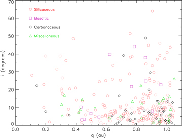
Figure 6. Distribution of PHA groupings in perihelion and inclination.
Download figure:
Standard image High-resolution image
Figure 7. Distribution of PHA groupings in semimajor axis and eccentricity.
Download figure:
Standard image High-resolution image
Figure 8. Distribution of PHA groupings in aphelion and Tisserand parameter with Jupiter.
Download figure:
Standard image High-resolution image
Figure 9. Distribution of PHA groupings in Earth MOID and absolute magnitude.
Download figure:
Standard image High-resolution imageThe median Earth MOID (Table 5; Figure 9) of the carbonaceous PHAs is also the lowest within the four groupings we identified (again, possibly because of observational biases). Considering that their relatively low inclinations will bring them to have more close approaches with the Earth, together with the fact that the most promising techniques for deviating a small body from hazardous trajectories are much less efficient for the (low-density, porous) carbonaceous objects (e.g., Perna et al. 2013a), these PHAs might pose a special hazard to our planet.
A relatively low value of the median Earth MOID is also found for the basaltic grouping. The median values that we obtained for the orbital parameters of V-type PHAs are consistent with the ranges of values that were found by Migliorini et al. (1997), who studied the dynamical routes from (4) Vesta (supposed to be the parent body of most/all of the V-type NEOs) to the near-Earth regions. Notably, all of the V-type NEOs show surfaces that are weakly affected by the "space weathering" (Fulvio et al. 2016; Ieva et al. 2016), which could be interpreted as being due to frequent close encounters with the Earth "refreshing" their surfaces (the same mechanism has been proposed by Binzel et al. 2010 to explain the unweathered surfaces of the Q-type NEOs). Hence the V-type PHAs also seem to deserve special attention in terms of impact risk mitigation analyses, although their mineralogy—apart from a higher content of pyroxene—is quite similar to that of the most common S- and Q-types.
5.2. Taxonomy versus Rotational Properties
Figure 10 presents the distributions of the spin period and of the light-curve amplitude of the PHA population (for some objects for which multiple solutions are given in the EARN database, we took the average values). Figure 11 shows a closer view toward the shorter rotational rates, where the "spin barriers" for cohesionless (i.e., held together by self-gravitation only) objects of different densities are also shown for reference (Pravec & Harris 2000). An asteroid of a given density, rotating faster than the corresponding spin limit, should be a monolith or have some internal cohesive strength to be held together against centrifugal break-up, e.g., due to van der Waals forces (Sánchez & Scheeres 2014). Conversely, objects spinning lower than this limit are expected to probably have a gravity-dominated structure.
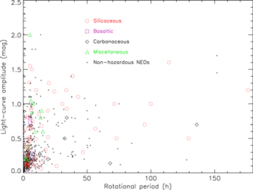
Figure 10. Distribution of PHA groupings in rotational period and light-curve amplitude.
Download figure:
Standard image High-resolution image
Figure 11. Distribution of PHA groupings in rotational period and light-curve amplitude: a zoom toward the faster spins. The rotational break-up limits for cohesionless bodies are also reported for different densities (from Pravec & Harris 2000).
Download figure:
Standard image High-resolution image
No clear correlation seems to exist between the rotational properties and the absolute magnitude of the objects, though extremely slow rotators are missing within the smallest population (Prot < 25 hr for H > 20, but observational biases should be taken into account). Note the presence of a not-so-small object (2011 XA3, with H = 20.5) within the very fast rotators (Prot = 0.73 hr), indicating that such an asteroid could represent a very challenging target in terms of risk mitigation activities. The other very fast rotators in the PHA population are 2011 BT15 (Prot = 0.11 hr, H = 21.8), 1998 WB2 (Prot = 0.31 hr, H = 21.8), and 2002 NV16 (Prot = 0.91 hr, H = 21.4).
In agreement with literature results on the asteroid rotational properties, the fastest rotators (Prot ≲ 5 hr) tend to acquire more spheroidal shapes with increasing spin rates, due to mass loss that can eventually lead to binary asteroid formation (e.g., Walsh et al. 2012).
However, for rotational periods ≳5 hr, and up to ∼80–90 hr, the opposite trend possibly appears, with more spheroidal shapes associated with the objects spinning more slowly. This could suggest different internal strengths with respect to the fast-spinning population, and/or different equilibrium shapes. Tanga et al. (2009) have found that "rubble pile" asteroids (i.e., gravitational aggregates with negligible internal strength) have the tendency to rapidly move toward fluid equilibrium shapes, producing more elongated objects with increasing spin frequency. They also found that at angular spin frequency  where G is the gravitational constant and ρ is the density, the equilibrium shape changes from elongated Jacobi ellipsoids (for fast rotators) to flattened Maclaurin spheroids (for slow rotators). For a typical asteroid density of 2.5 g cm−3, such "critical" spin corresponds to a rotational period of ∼4.5 hr, which is notably close to the observed elongation maximum at Prot ∼ 5 hr.
Such anti-correlation between the rotational period and the maximum light-curve amplitude (Δm), if real, should in principle be followed by the whole NEO population, and not only by PHAs: actually, non-hazardous NEOs seem to follow the same trend (Figure 10). We tried to verify if this correlation actually exists, binning the objects in 10 hr Prot intervals, and checking the maximum value of the Δm for each bin: considering the range Prot = 0–90 hr, we obtain a Pearson correlation coefficient of r = −0.928. The probability that nine measurements (i.e., the number of bins) of two uncorrelated variables would yield  0.928 is about 0.03% (e.g., Taylor 1997), so the trend can be considered statistically significant. Considering the range 0–80 hr (8 bins), we obtain r = −0.900, and a non-correlation probability of 0.2%. Discarding objects with Prot < 5 hr, or taking 5 hr bins in the 5–20 hr range, does not change our results in a significant way.
For rotational periods longer than about 80–90 hr, the anti-correlation with the light-curve amplitude seems to disappear, and some elongated very slow rotators are present. This possibly different regime could be related to the YORP effect (the torque produced by anisotropic thermal emission, which can be important for NEOs) and small collisions. Marzari et al. (2011) have shown that the combined effect of these processes can cyclically change the rotational period of asteroids (from hours to hundreds of hours, and vice versa), over timescales compatible with the dynamical lifetime of NEOs (≈106 years). The same authors have also shown that for asteroids in a slow rotation state, small-scale collisions can temporarily halt the YORP evolution, triggering a period of slow rotation characterized by a random walk in the spin period.
What is detailed above is based on a very limited data set, so further observational and theoretical work is strongly required to test our estimates. We also stress that for such very long rotational periods, an observational bias against the discovery of the less elongated shapes clearly exists, so one could predict that the lower part of Figure 10 is much more densely populated than it currently appears.
As for the differences in terms of rotational properties between the four compositional groupings that we defined, it seems that these obey "different spin barriers" (Figure 11). In this sense, as expected, the carbonaceous PHAs are the most fragile, while the two most extreme rotators (Prot ∼ 2 hr, Δm ∼ 0.2 mag), within their plausible spin barrier, are the Xe-type (144898) 2004 VD17 and the X-type (29075) 1950 DA. The former has already been demonstrated to have an important internal strength by De Luise et al. (2007), while the latter has been found to have enstatitic or metallic nature (Rivkin et al. 2005).
The miscellaneous (i.e., mostly X-type) PHAs also show the highest median light-curve amplitude, with (367248) 2007 MK13 having the largest absolute value (Δm = 2 mag): its X-type spectrum is inconclusive in determining the composition of this body, but its albedo value (0.119) suggests a "metallic" nature.
Conversely, the carbonaceous PHAs have the lowest median light-curve amplitude, and no objects with Δm > 0.3 mag for rotational periods lower than ∼30 hr, again suggesting lower cohesive strengths. Notably, the carbonaceous PHAs also present a considerably slower median rotational period than the other groupings, though we stress that discarding the slowest rotator of such population ((53319) 1999 JM8, Prot = 136 hr), the median value is lowered from 7.15 to 5.95 hr.
6. SUMMARY AND CONCLUSIONS
In this paper we present new spectroscopic observations of 14 PHAs, for which we determined the taxonomic classification, meteorite spectral analogs, and mineralogy.
After combining our results with the available literature, we found that the taxonomic distribution of PHAs is similar to that of NEOs in general (i.e., dominated by the S/Q complex, though observational biases surely affect such distribution). Given a number of uncertainties about their taxonomy and composition, we defined four "groupings" of objects: the "silicaceous" (types S, Q, A, and O), the "basaltic" (V-types), the "carbonaceous" (types B, C, D, P, T, and Xc), and the "miscellaneous" (types X, Xe, Xk, K, and L) PHAs. Then we analyzed the distribution of such groupings in terms of dynamical and physical properties.
The primitive, carbonaceous asteroids seem to pose a special danger to our planet: not only are the most mature techniques for deviating an asteroid from a hazardous orbit less efficient for such objects (e.g., Perna et al. 2013a), but their low MOID and inclination values indicate that these PHAs will have close approaches with the Earth more frequently than those belonging to the other groupings. Based on their low albedo and Tisserand parameter, we also identified two candidate extinct cometary nuclei within the carbonaceous PHAs, which could present extremely low porosities: 2001 XP1 and 2002 BM26. The possible cometary origin of 2001 ME1 and (4015) Wilson–Harrington was already pointed out in previous works.
The basaltic PHAs also deserve special attention, as the dynamical routes from Vesta to the near-Earth region seem to put them on orbits characterized by low MOID values and frequent close approaches with our planet, as also suggested by the latest findings about the lack of space weathering on the surfaces of V-type NEOs.
Because of their rapid rotations and elongated shapes, suggesting an important internal strength, additional objects that we identified as particularly hazardous are the silicaceous 2011 XA3, 2011 BT15, 1998 WB2, and 2002 NV16. The X-types (29075) 1950 DA and (367248) 2007 MK13 also deserve attention because of their possible metallic nature and extreme rotational properties (as well as the Xe-type (144898) 2004 VD17). Conversely, no fast rotators are found within the carbonaceous PHAs, suggesting low cohesions.
Finally, we identified a possible trend that might be followed by PHAs and NEOs in general, with more elongated shapes associated with shorter rotational periods in the range Prot ≈ 5–80 hr. This seems to be in agreement with the predicted behavior of gravity-dominated bodies assuming spheroidal shapes to maintain the rotational equilibrium (e.g., Tanga et al. 2009). The opposite trend was already known to exist for Prot ≲ 5 hr, due to rotational break-up. However, for rotational periods that are longer than about 80–90 hr, no correlation seems to exist with the shape, although the statistics is very low. Further observational and theoretical work will be necessary to understand the reason for such a "third regime" emerging among the slowest rotators. Possibly, both the YORP effect and collisions may play a role in this scenario (e.g., Marzari et al. 2011). More observational data will allow us to check for the existence of different behaviors among objects of different taxonomy/composition, possibly helping to determine the physical motivation of such regime.
We thank Driss Takir, the referee of our manuscript, for his positive reception and valuable comments. D.P. thanks Paolo Tanga for the stimulating discussions about the rotational properties of asteroids. D.P. and S.I. acknowledge financial support from the NEOShield-2 project, funded by the European Commission's Horizon 2020 program (contract No. PROTEC-2-2014-640351). S.I. also acknowledges financial support from ASI (contract No. 2013-046-R.0: "OSIRIS-REx Partecipazione Scientifica alla missione per la fase B2/C/D"). Part of the data utilized in this publication were obtained and made available by the MIT-UH-IRTF Joint Campaign for NEO Reconnaissance. The IRTF is operated by the University of Hawaii under Cooperative Agreement no. NCC 5-538 with the National Aeronautics and Space Administration, Office of Space Science, Planetary Astronomy Program. The MIT component of this work is supported by NASA grant 09-NEOO009-0001, and by the National Science Foundation under grant Nos. 0506716 and 0907766.
Facilities: IRTF - Infrared Telescope Facility (SpeX - ), NTT - New Techology Telescope (EMMI - , SofI - ), TNG - Telescopio Nazionale Galileo (DOLORES - , NICS - ).
Footnotes
- 10
- 11
- 12
- 13
- 14
http://earn.dlr.de; retrieved on 2015 April 28.