
Abstract
Porous electrodes are prevalent in electrochemical devices. Electrochemical impedance spectroscopy (EIS) is widely used as a noninvasive, in situ characterization tool to investigate multi-phase (electronic, ionic, gaseous) transport and coupling interfacial reactions in porous electrodes. Interpretation of EIS data needs model and fitting which largely determine the type and amount of information that could possibly be obtained, and thereby the efficacy of the EIS method. This review focuses on physics-based models, as such models, compared to electrical circuit models, are more fundamental in our understanding of the porous electrodes, hence more reliable and more informative. Readers can have a glimpse of the long history of porous electrode theory and in particular its impedance variants, acquaint themselves with the celebrated de Levie model and a general theoretical framework, retrace the journey of extending the de Levie model in three directions, namely, incorporating new physico-chemical processes, treating new structural effects, and considering high orders. Afterwards, a wealth of impedance models developed for lithium-ion batteries and polymer electrolyte fuel cells are introduced. Prospects on remaining and emerging issues on impedance modelling of porous electrodes are presented. When introducing theoretical models, we adopt a "hands-on" approach by providing substantial mathematical details and even computation codes in some cases. Such an approach not only enables readers to understand the assumptions and applicability of the models, but also acquaint them with mathematical techniques involved in impedance modelling, which are instructive for developing their own models.
Export citation and abstract BibTeX RIS

This is an open access article distributed under the terms of the Creative Commons Attribution 4.0 License (CC BY, http://creativecommons.org/licenses/by/4.0/), which permits unrestricted reuse of the work in any medium, provided the original work is properly cited.
The ongoing paradigm shift in energy technology causes rising and falling in many research fields. 1,2 Transport in porous media is a particular research field of which the importance is unattenuated during the paradigm shift, because it is a commonality shared by fossil and renewable energy technologies. 3,4 For instance, a key issue of petroleum engineering is fluid flow through porous media. 5 As for renewable energy technologies, such as secondary batteries, fuel cells, and supercapacitors, transport in porous electrodes, which are employed for the sake of enlarging the electrochemical active surface area and thus magnifying the energy and power density of the device, is a fundamental process. 4,6,7 Moreover, the advent of various renewable energy technologies broadens the scientific content of porous media, triggering a surge of interest in understanding multi-scale, multi-phase, multi-component (neutral and charged) transport processes that are coupled with a variety of bulk and interfacial reactions. 4,7,8
Compared to its counterparts in rocks and soil, a porous electrode features an electrified interface between the solid matrix and the electrolyte solution filling, partially or fully, the pore network. The electrified interface brings into play complicated interactions between charge transport in the solid matrix and that in the electrolyte solution. The interactions pose additional challenges to attacking the problem, but it also brings new possibilities. For one, we are now able to "probe" the porous electrode by means of electrical signals. Out of many variants of electrical methods, electrochemical impedance spectroscopy (EIS) has the merits of a noninvasive nature and high temporal resolution.
9–11
In its standard form, the EIS method imposes a sinusoidal voltage perturbation with a small magnitude of 5 ∼ 20 mV and an angular frequency  onto the porous electrode under investigation, measures the current generated from reactions and transport processes that are "activated" by the perturbation, and then calculates impedance response via Fourier transform. By varying
  one is able to "probe" physico-chemical processes of interest in a wide frequency range readily extending over ten orders nowadays.
The challenge does not end with obtaining EIS data, but just begins, instead. Models are needed to interpret the EIS data. Most often, electrical equivalent circuits (EECs) are employed to analyze EIS data. Albeit being simple, generic, and readily accessible in commercial softwares, the EEC approach suffers from the "polysemy," namely, the same piece of EIS data can be fitted, within experimental accuracy, with several EECs of different physical implications. 12,13 In Macdonald's words, "EECs are analogs not models." 12 The polysemy of the EEC approach is transferred, unfairly, to the EIS method, which is sometimes regarded as uncertain, subjective, and intangible. To crush such misconception and to realize the full potential of the EIS method, physical models, together with well-controlled experiments, are in need. The need is even more acute for porous electrodes than extended electrochemical interfaces, as the nonhomogeneous polarization in porous electrodes outreaches the capabilities of simple EECs.
Despite of its necessity and power, the physics-based modelling approach is much less practiced in the literature. We believe that a tutorial review on this topic will help spread its usage. We give a brief sketch of the history background in the section of 'Historical Notes', revisit the classical de Levie model in the section of 'de Levie Impedance Theory', recapitulate extensions made to the de Levie model in three directions (physics, structure, and order) in the section of 'Theoretical Progress', illustrate its applications to lithium-ion batteries and fuel cells in the section of 'Selected Applications', and prospect its future development in the section of 'Prospect for Future Development'. With the purpose and hope that this review may well be used as a tutorial tool, we usually start with presenting a general theoretical framework, provided with substantial mathematical details, and then review previous studies in the context of the presented framework. This arrangement is designed to improve the logic, accessibility and completeness in the exposition of theoretical works. The pursuit of logic completeness impels us to include unpublished results in some cases, for example, the impedance model of solid-electrolyte interphase.
Given the vast amount of research works in the past decades, this review is by no means comprehensive. For a general introduction of EIS, readers are referred to several monographs. 9–11,14,15 For reviews specialized on electrochemical interfaces, readers shall consult Chang and Park, 16 Bandarenka, 17 Pajkossy and Jurczakowski, 18 and Huang. 19 There are a dozens of reviews about EIS applications to lithium-ion batteries, 20 fuel cells, 21,22 and other electrochemical devices. 23,24 Lasia published a book chapter on modeling of impedance of porous electrodes in 2009 25 and extended the discussion in a recent book, 15 which are of closest relevance to this review. The present review can be regarded as a complement to the ones written by Lasia.
Historical Notes
Yai Sakizo invented zinc-carbon batteries in 1887. 26 Three years later, Mond and Langer developed Grove's idea and built the first practical H2/O2 fuel cell using a porous Pt electrode. 27 Since then, one of the oldest questions asked by electrochemical engineers is: where is the more active part of the porous electrode? In 1945, Coleman, a battery engineer from Burgess Battery Company, presented his mathematical models to analyze the current and potential distributions in a porous cathode of zinc-carbon batteries in front of the attendees of Ninetieth General Meeting of the Electrochemical Society. 28 At the very same meeting, Weisselberg independently reported a mathematical model to simulate current distribution along the cylindrical anode during electroplating. 29
At the infancy of electrochemical modeling, Coleman and Weisselberg, two pioneers in this field, were very humble with their contributions. Coleman described his straddle toward calculation of battery performance from principles of physics as "trivial" and "cannot compete with a test laboratory." 28 In addition, Coleman was worried that the messy mathematical expressions would frighten his readers, and scrupulous about the simplifications made in the "crude model" (so described by himself). There were also encouraging comments. James Waber commented in the discussion section of Weisselberg's paper that "Weisselberg deserves special credit for applying differential equations to the solution of a practical problem such as electroplating," and advocated that "His success should convince others of the practicability of such a study." 29
In hindsight, physical principles required to describe electrochemical processes in porous electrodes were readily at hand decades earlier. Kirchhoff's circuit laws have been known since 1845. 30 Adolf Fick published the law of diffusion in 1855. 31 The edifice of electrode kinetics had been established by Butler, Volmer, and Erdey-Grúz in 1920s. 32 However, according to the retrospect of Bockris, the atmosphere of electrochemistry in 1940s was dominated by "the dead hand of Nernst," namely, thermodynamic analysis. 33 It then comes as no surprise that electrochemical modeling was an act of eccentricity in 1940s.
A group of Russian electrochemists independently developed porous electrode theory around the same time. Leading authors are Frumkin, 34 Daniel-Bekh, 35 Ksenzhek and Stender. 36 Readers can consult Grens and Tobias, 37 Breiter, 38 and Posey 39 for these early Russian works. The Russian school systematically studied current and potential distributions along the longitudinal direction in porous electrodes, with different descriptions of interfacial reactions (linear, Tafel, or Butler-Volmer equations) and different pore geometries (finite and semi-infinite). It is worth noting that Daniel-Bekh proposed transmission line representation of porous electrodes in 1948. 35
The next major step was made by Newman and Tobias in 1962. 40 Different from previous works treating a single pore, Newman and Tobias developed a macrohomogenous theory which describes the porous electrode, interspersed by multiple phases, as a homogeneous medium with averaged physico-chemical properties. Additionally, Newman and Tobias consistently accounted for the effect of mass transport on electrochemical reactions. 40
The year 1963 ushered in a milestone made by de Levie for both porous electrode theory and electrochemical impedance spectroscopy (EIS). 41 In the celebrated tetralogy of porous electrodes in electrolyte solutions, de Levie systematically studied current (potential) distribution in a uniform semi-infinite pore under potentiostatic (galvanostatic) and potentioharmonic (galvanoharmonic) conditions, allowing analytical solutions in the ac regime. 41–43 It should be mentioned that Ksenzhek and Stender had published ac response of porous electrodes in 1956, 36 seven years before de Levie. However, it is a fact that de Levie's paper opens up the research field of impedance response of porous electrodes, whereas the paper of Ksenzhek and Stender, written in Russian, has restricted impact around the world.
In the decades succeeding de Levie's seminal work, abundant research activities greatly deepen and widen the research field of impedance response of porous electrodes. 25,38 As depicted in Fig. 1, these research activities are categorized into three threads, namely, extension in physics, extension in structure, and extension from linear to nonlinear regime.
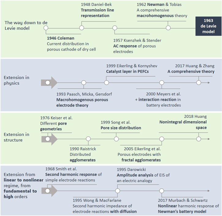
Figure 1. Historical overview of theory of impedance response of porous electrodes with an emphasis on the ac response.
Download figure:
Standard image High-resolution imageIn its most widely cited version, de Levie model treats a capacitive interface along the cylindrical pore. 41 Nevertheless, in the original papers, de Levie also considered Faradaic reactions at the interface, as well as axial and radial diffusion of species in solution. 41–43 Consequently, de Levie's original treatment is very comprehensive. In later developments, researchers emphasized certain aspects of the problem. For example, Darby, 44,45 Keddam, Rakotomavo, and Takenouti 46 emphasized the importance of axial diffusion. In 1993, Paasch, Micka, and Gersdorf derived the impedance response of a porous electrode based on a comprehensive macrohomogenous porous electrode theory. 47 This work includes ionic conduction in the electrolyte phase and electronic conduction in the electrode phase, double layer charging and Faradaic reactions at the interface, and diffusion. In 1999, Eikerling and Kornyshev developed a detailed impedance theory of fuel cell electrodes based on the macrohomogenous porous electrode theory, which is widely used in characterization and diagnosis of fuel cells. 48 In 2000, Meyers et al. developed impedance models for lithium-ion battery electrodes. 49 Very recently, Huang and Zhang developed a comprehensive theoretical framework for impedance response of porous electrodes with different types of electrochemical interfaces (blocking electrode, electrode with faradaic reactions, and electrode constituted of particles with insertion reactions), treated in-plane, through-plane and multi-dimensional inhomogeneities, and obtained analytical solutions for the full case and four limiting cases as well. 50
The second direction of extension aims to study structural effects. In 1976, Keiser, Beccu, and Gutjahr studied the impedance response of a single pore with different shapes. 51 In 1990, Raistrick modelled the impedance response of a fuel cell electrode made up of agglomerates. 52 For this case, the electrochemical interface distributed along the pore is replaced with distributed agglomerates covered with a thin film. In-plane distribution of the pore size was treated by Song et al. 53 in 1999, resulting in an inclined line in low frequency range. When modeling the impedance response of carbon-based double layer capacitors, Eikerling, Kornyshev and Lutz further extended the distributed impedance elements along the macroscopic pore by considering distributed agglomerates with a fractal microscopic pore structure. 54 Recently, Huang treated mass transport in a porous electrode with nonintergal dimensionality using fractional calculus. 55
The third direction of extension goes beyond the linear regime and studies the impedance response of porous electrodes under nonlinear conditions. In addition to the fundamental-order impedance response, higher-order impedance response can be obtained in nonlinear regime. This direction of research has captivated interest in the characterization and diagnosis of fuel cells and batteries. 56–58 In 2017, Murbach and Schwartz simulated the nonlinear impedance response of lithium-ion batteries described by Newman's battery model. 59 Earlier interest in high-order impedance response dates back to 1960s when Smith studied the second harmonic response of simple electrode reactions. 60,61 In 1995, Wong and MacFarlane obtained the second harmonic impedance of electrode reactions with diffusion. 62 Around the same time, Darowicki investigated the nonlinear effects on electrochemical impedance by analyzing the amplitude dependence of EIS of an electric analogy. 63
de Levie Impedance Theory
In this section, we revisit the celebrated classical de Levie model published in 1963. This revisit, on the one hand, may help readers to get familiar with impedance modelling, on the other hand, is instrumental to the enunciation of the assumptions and applicability of de Levie model. 15,64 Preliminaries of impedance modelling are provided the supporting information (SI is available online at stacks.iop.org/JES/167/166503/mmedia) of this article. Please refer to Table I for the list of symbols used in this section. Readers are also referred to Lasia for a pedagogical exposition of the de Levie model. 15
Table I. List of symbols in section 'de Levie Impedance Theory'.
| Symbol | Description |
|---|---|

| Double-layer capacitance, F m−2 |

| Potential perturbation, 
|

| Current in the electrolyte phase, 
|

| Total current flowing through the porous electrode, 
|

| Length of the pore, 
|

| Total number of the pores |

| Radius of the pore, 
|

| Resistivity of the electrolyte phase, 
|

| Total electrolyte resistance of the pore, 
|

| Solution resistance outside the pores, 
|

| Impedance of the double layer, 
|

| Double layer impedance per unit length, 
|

| Impedance of the pore, 
|

| Total impedance of the pores, 
|

| Penetration length, 
|

| Electronic resistivity, 
|

| Ionic resistivity, 
|

| Electrolyte phase potential, 
|

| Solid phase potential, 
|

| A dimensionless variable, 
|
In the de Levie model, the porous electrode is treated as circular cylindrical channels of uniform diameter and of semi-infinite length, as depicted in Fig. 2a. The pore wall is made of materials with infinite electrical conductivity, namely, the electronic resistivity  The pore is filled homogeneously with supporting electrolyte characterized by ionic resistivity
  (
( ). In the axial direction, ion migration is described using the Ohm's law.

Figure 2. (a) Treatment of porous electrodes as a parallel collection of uniform cylinder pores; (b) The equivalent electrical circuit of a cylindrical pore with uniformly distributed electrolyte resistance Re, and the specific impedance of the interface between electronic and electrolyte phase, Zdl; (c) Impedance of a porous electrode in the Nyquist plot.
Download figure:
Standard image High-resolution imageRobert de Levie sets himself the task of obtaining the potential and current distributions as a function of the coordinate z along the central axis of the cylinder and time  when the pore is subject to various kinds of potential/current stimulus. The original treatment of de Levie is somewhat cumbersome, which can be much simplified by the aid of Fourier transform (a rudimentary introduction is provided in the SI of this article). In subsequent development in this section, all Fourier-transformed variables are marked with an over-tilde.
Figure 2b depicts the equivalent electrical circuit of the porous electrode. The upper line corresponds to the electronic phase, of which the electronic resistivity is zero. The bottom line corresponds to the electrolyte phase, of which the resistivity is  (
( ). The total electrolyte resistance of the pore reads
  The specific impedance of the interface between electronic and electrolyte phase is denoted as, generally,
  (
( ). For a non-Faradaic interface with a double-layer capacitance of
  (F m−2), we have,
  with
with  being the angular frequency. The interfacial impedance per unit length (pul) is then given by,
Between two nodes connected by an ionic resistance of  the potential difference is given, according to the Ohm's law in frequency domain, by,
  which is changed to a differential equation,
At each node, the current change,  is equal to the current flowing from the electronic phase to the solution phase, which is given by,
  yielding,

Differentiating Eq. 1 with  combining it with Eq. 2, and assuming there is no potential gradient in the electronic phase, namely,
  we have

which is closed with following boundary conditions. A potential perturbation, of which the Fourier-transformed counterpart is denoted  is imposed on the porous electrode, namely,
  As
As  we have

At the other pore end, electrical current in the electrolyte phase cannot penetrate into the pore wall, namely, the electrical current is zero at 

The solution of Eq. 3 closed with relevant boundary conditions is written as

The total current density flowing through the porous electrode is calculated at  which, according to Eqs. 1 and 6, is written as
Impedance of the pore is defined as the ratio of the Fourier-transformed potential with respect to the Fourier-transformed current density,

which is rearranged into a more concise and general form,

where  is a dimensionless variable representing the relative importance of electrolyte-phase resistance compared to the interfacial impedance. For a non-Faradaic interface, we have,
  As a result, the magnitude of
  increases as
  increases. At very high frequencies such that,
  we have
  and
and

which indicates that both real and imaginary parts of  are proportional to
  namely, the impedance is manifested as a 45° line in the Nyquist plot, as shown in Fig. 2c. That the magnitude of
  decreases as
  increases is ascribable to the fact that a smaller part of the pore is penetrated by a perturbation with a higher frequency.
At very low frequencies such that  we have
  and
and

which results in,  for a non-Faradaic interface. The impedance is manifested as a vertical line in the Nyquist plot, as shown in Fig. 1c.
If there are  pores in parallel and there is a solution resistance of
  outside the pores, the total impedance of the pore assembly is given by

The frequency-dependence of  is elucidated in a clearer way by defining a frequency-dependent penetration length
  characterizing the effective perturbing length of a sinusoidal perturbation with an angular frequency of

which is equal to  for a non-Faradaic interface. It is readily seen that
  is larger when
  is smaller, namely, a slowly alternating signal results in a deeper perturbation. As
  decreases,
  increases, implying that the pore is now fully accessible to ac signal and the electrolyte-phase resistance thus grows. When
  becomes larger than the pore length, meaning that the whole pore is now fully "activated," further decrease in
  does not change the electrolyte-phase resistance any longer. In such case, variation in the pore impedance is dominated by the interfacial impedance, resulting in a vertical line in the impedance plot.
The standard de Levie model, despite of its simplicity, captures an essential characteristic of the impedance response of porous electrodes, that is, the 45° line in high frequency range in the Nyquist plot, of which the physical meaning is a frequency-dependent electrochemical surface area. This becomes a signature of porous electrodes. In addition, the real part of low-frequency impedance is simply,  providing a simple approach to measure the ionic conductivity of the electrolyte and the pore structure parameters. However, full awareness of the assumptions of the de Levie model should be present in practical applications; they are:
- (1)The porous electrode is treated as a collection of one-dimensional and homogeneous (in terms of transport, interfacial, and structure properties) cylindrical pores in parallel connection. Its extension to non-homogeneous cases with other pore structures will be discussed in the section 'Extension in structure'.
- (2)The electrode-electrolyte interface is purely capacitive. No charge-transfer reaction is considered. This assumption is valid for porous electrodes of genuine supercapacitors, but fails for porous electrodes of lithium-ion batteries (LIBs) where intercalation/deintercalation reactions occur, 49,65–70 and for porous electrodes of polymer electrolyte fuel cells (PEFCs) where oxygen and hydrogen reactions occur. 39,48,71–74 One can use non-intercalating electrolyte or totally reflecting pore wall to permit the usage of de Levie model for LIB porous electrodes. As for PEFCs, the EIS measurement should be conducted in the double-layer charging region under H2/N2 gas condition. Extension to complex electrode-electrolyte interfaces will be discussed in the section 'Extension in physics: a theoretical framework'.
- (3)The pore wall is made of materials with infinite electrical conductivity. This assumption is well realized in carbon-based/supported porous electrodes for supercapacitors, LIBs and PEFCs. Otherwise, the resistance due to electron transport in the solid phase should be accounted for, which will be discussed in a general theoretical framework presented in the section 'Extension in physics: a theoretical framework'.
- (4)In the axial direction, only ion migration is described using the Ohm's law. Ion diffusion driven by concentration gradient is neglected. In addition, the influence of concentration distribution on the interfacial capacitance is not considered. This assumption is hardly met in practical situations where mass transport and its coupling with interfacial reactions are present. We will amend this assumption in a general theoretical framework presented in the section 'Extension in physics: a theoretical framework'.
- (5)There is no dc current flowing through the porous electrode, otherwise the impedance response can be calculated numerically only. In addition, it is a linear response theory concerning the fundamental-order impedance response only. Its extension to the nonlinear regime and higher-order impedance response will be discussed in the section 'Extension in order'.
Theoretical Progress
Extension in physics: a theoretical framework
The standard de Levie model is based on simple physics: a capacitive interface, neglect of electrical conduction in the solid phase, and description of charge transport in the solution phase using the Ohm's law. Continued efforts have been conducted to extend the standard de Levie model by adding more physics into it. This section recapitulates research progress in this direction. Our exposition unfolds in a hands-on way. W e start by constructing a theoretical framework of impedance responses of porous electrodes in several steps. First, ion transport in the intrinsic electrolyte phase is formulated by adopting a phenomenological free-energy approach. Second, the structure information of the porous electrode is incorporated into the intrinsic equations via the volume averaging method and coordinate transformation. Third, impedance expressions are derived for general and several limiting cases. Readers familiar with porous electrode theory can safely skip the first three subsections. Afterwards, we contextualize previous studies within this theoretical framework. Please refer to Table II for the list of symbols used in this section.
Table II. List of symbols in section Extension in physics: a theoretical framework.
| Symbol | Description |
|---|---|

| A quantity in the porous electrode |

| Intrinsic liquid-phase average of 
|

| Fluctuation of 
|

| Volumetric electrochemical surface area, 
|

| Molar enthalpy of cations (+) and anions (−), 
|

| Concentration of cations (+) and anions (−), 
|

| Electrolyte concentration under electroneutrality condition, 

|

| Fourier-transformed concentration, 
|

| Total concentration of ions, 

|

| Li+ concentration in the solid phase, 
|

| Double layer capacitance, F m−2 |

| Diffusion coefficients of cations (+) and anions (−), 
|

| Effective diffusion coefficient, 
|

| Solid-phase diffusion coefficient, 
|

| Sinusoidal voltage perturbation, 
|

| Activity coefficient of cations (+) and anions (−) |

| Current stimulus, 
|

| Current density of cations (+) and anions (−)in the electrolyte phase, 
|

| Total current density in the electrolyte phase, 

|

| Fourier-transformed total current density, 
|

| Characteristic length of microscopic heterogeneities |

| Thickness of the porous electrode, 
|

| Characteristic scale of the porous electrode, m |

| Characteristic scale of RVE |

| Mobility of cations (+) and anions (−), 
|

| Flux of cations (+) and anions (−), 
|

| A constant with the dimension of 
|

| Average radius of solid active particles, 
|

| Radius of the active particles, 
|

| Charge transfer resistance, 
|

| Solution resistance out of the pore, 
|

| Ion transference number of cations (+) and anions (−) |

| A constant,  or temperature, or temperature, 
|

| Average molar volume of ions, 
|

| Velocity of interface, 
|

| Characteristic volume of RVE, m3 |

| Liquid volume, m3 |

| Charge number of ions, 
|

| Local impedance at the EEI, 
|

| Impedance of porous electrode, 
|

| Exponent of a CPE |

| Liquid volume fraction |

| Volume fraction of solid active particles |

| Effective electronic conductivity, 
|

| Effective ionic conductivity, 
|

| Electrochemical potential of ions, 
|

| Constant in electrochemical potential expressions, 
|

| Ion conductivity of cations (+) and anions (−), 
|

| Total conductivity of electrolyte, 

|

| Effective conductivity, 
|

| Frequency-dependent ac conductivity, 
|

| Local tortuosity |

| Crossover frequency |

| Exponent of a CPE |

| Electric potential in the electrolyte phase, 
|
Theory of ion transport in electrolyte
The electrolyte solution is assumed to be binary and symmetric. Therefore, under the premise of electroneutrality condition, the concentrations of cations and anions are equal,  The electroneutrality assumption is valid if the characteristic size of the volume containing the electrolyte solution is much larger than the Debye length which is proportional to
  and equal to 0.96 nm for an aqueous strong electrolyte of 0.1 M.
75
Ion transport takes place via diffusion and migration, while the convection effect is neglected. Consideration of natural convection using a modified Poisson-Nernst-Planck theory can be found in Ref. 76. We further assume there is no chemical reaction in electrolyte. A general theoretical framework considering chemical reactions and mechanical effects has been developed by Dreyer et al.
77,78
and equal to 0.96 nm for an aqueous strong electrolyte of 0.1 M.
75
Ion transport takes place via diffusion and migration, while the convection effect is neglected. Consideration of natural convection using a modified Poisson-Nernst-Planck theory can be found in Ref. 76. We further assume there is no chemical reaction in electrolyte. A general theoretical framework considering chemical reactions and mechanical effects has been developed by Dreyer et al.
77,78
According to the lattice-gas model, the electrochemical potential of ions in electrolytic solution considering the ion size effect is expressed as 79

where  and
and  are the molar enthalpy of cations (+) and anions (−),
  and
and  are the concentration of cations (+) and anions (−),
  and
and  refer to the total concentration and average molar volume of ions, respectively.
  and
and  have their usual meanings. If we assume that electrostatic interactions described in a mean-field manner dominate over short-range forces in the electrolyte solution, we have
  with
with  being an unspecified constant with trivial importance here,
  the charge number of ions, and
 Faraday constant, and
  the electrostatic potential in the electrolyte phase.
Microscopically, ion transport has been described as a vacancy-coupled ion transfer reaction. 80,81 Within this picture, the mass conservation law of ion transport is written as

where  are the diffusion coefficients of cations (
 ) and anions (
 ), respectively. Compared to its usual form, Eq. 15 features the term
  which is the direct consequence of the steric effect.
Substituting Eq. 14 into the flux term gives

The ionic conductivity is defined as,  where
where  is the mobility. The relationship between diffusion coefficient and mobility is given by Einstein's relation,
  Equation 16 is then rewritten as


where we have used the electroneutrality assumption which prescribes  and
and  for a binary symmetric electrolyte.
The total conductivity of electrolyte  is the sum of cationic and anionic conductivity,
  The ion transference number, representing the contribution of a sort of ion to the total ionic conductivity, is given by,
  respectively. The total current density in the electrolyte phase is carried by both cations and anions, given by,
  which is expanded as
It is readily seen from the above formula that the current density in electrolyte is driven by the potential gradient via migration, and together by the concentration gradient via diffusion. For the case of  the contribution driven by concentration gradient disappears. In addition, for the case of diluted solution, we have
  and Eq. 19 reduces back to the Ohmic law used in the standard de Levie model.
64
and Eq. 19 reduces back to the Ohmic law used in the standard de Levie model.
64
By some algebra manipulation, we can represent ion fluxes in terms of collective electrolyte variables, namely,  and
and 


Substituting this flux expression back into the mass conservation law of, for example, anions, we obtain
Equations 19 and 22 are the basic equations which describes the charge conservation and the transport of ions in a symmetric binary electrolyte. Generally,  and
and  can be considered as a constant. Using Fourier transform, one can rephrase Eqs. 19 and 22 in terms of perturbed variations marked with an over-tilde

The major difference between the current formulation and the Newman theory exists in the electrochemical potential of ions. 4 In the Newman theory, Eq. 14 is replaced with

with a generic, unspecified activity coefficient,  which in the present theory is explicitly given by,
  considering the ion size effect.
Upscaling via volume averaging
The volume averaging method provides a means to account for the essential features of a porous electrode without going into exact geometric detail. 82,83 In this section, we upscale the microscopic electrolyte equations expressed in Eqs. 23 and 24 to macroscopic electrolyte equations with an average consideration of the complex porous structure.
Representative volume element (RVE) is a key concept in the volume averaging method.
84,85
The RVE is a characteristic volume  that is sufficiently large to effectively sample all microscopic heterogeneities, and is sufficiently small to serve as a volume element of the continuum media. In this regard, the RVE has a characteristic scale of
  satisfies

where  is the characteristic scale of microscopic heterogeneities, and
  is the characteristic scale of the porous electrode, as shown in Fig. 3a.
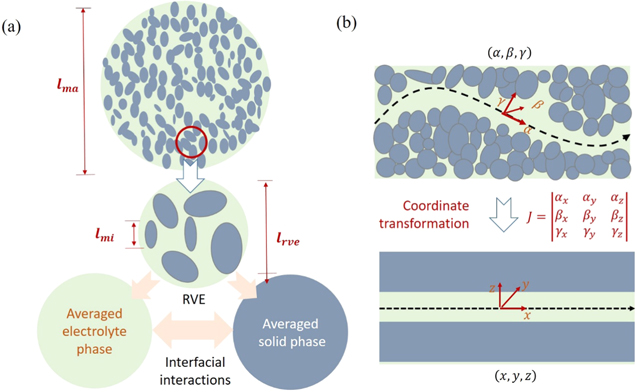
Figure 3. (a) Schematic illustration of the representative volume element in volume averaging method. (b) Local torturous coordinate  in the porous electrode and the transformed regular Cartesian dimension
Download figure:
Standard image High-resolution imageThe volume-averaged value of a property  over the volume
  is defined as

If  belongs only to the liquid volume
  we obtain

where  is the liquid volume fraction and
  is the intrinsic liquid-phase average of
  The fluctuation of
  is given by

By means of Leibniz's rule for differentiation under the integral sign, the volume averaged counterparts of the temporal derivative, gradient and divergence follow 86,87


where  is the velocity of interface,
  is a unit normal vector pointing outward from the phase under consideration. Eq.(30) is also termed Reynolds transport theorem in the field of fluid dynamics. If we neglect volume change,
  and the integral term on the right-hand side of Eq. 30 disappears.
The volume average of the product of two quantities is,

We neglect  in subsequent development, based on the assumption that the order of magnitude of the fluctuation is smaller than that of the average.
By this point, we are fully-fledged to derive macroscopic volume-averaged equations for ion transport in the electrolyte phase. We assume that only cations exchange between the electrolyte and solid phase through the interface, while the anion flux at the interface is zero. Therefore, substituting  with the Fourier-transformed cation flux
  and anion flux
  we have,


in the frequency domain. The source flux in Eq. 34 is further given by,

where  is the local impedance at the electrode/electrolyte interface (EEI),
  is the volumetric electrochemical surface area. If we assume that solid particles are spherical and all surfaces are electrochemically accessible, we have
  with
with  representing the volume fraction of solid active particles and
  their average radius.
Adding Eqs. 34 and 35, substituting  with
with  and using Eq. 36, one can obtain

The volume averaging of both sides of Eq. 23 yields
In addition, according to Eq. 31,  and
and  can be written as


Therefore, Eq. 38 can be rewritten as
Substituting Eq. 41 into Eq. 37, one can obtain the frequency-domain volume-averaged equation describing charge conservation in the electrolyte phase,
Similarly, we transform Eq. 24 to
Coordinate transformation
It should be noted that the divergence and gradient operators in Eqs. 42 and 43 are conducted in the local torturous space, denoted  and depicted in Fig. 3b. We now embark on transforming Eqs. 42 and 43 from the local coordinate
  to the regular Cartesian coordinate
  as depicted in Fig. 3b.
For a scalar quantity, say  the gradients in two coordinate systems are correlated as
65
the gradients in two coordinate systems are correlated as
65


where we follow Einstein summation convention, and the coordinate transformation matrix determinant  and coefficients
  are given by
where  indexes over (
 ) and
) and  is the unit vector in the (
 ) coordinate. For the one-dimension case, we have

where  is the local tortuosity.
Thereafter, Eqs. 42 and 43 in the regular Cartesian coordinate  are rewritten as,
which are the general equations of ion transport in the electrolyte phase in porous electrodes obtained via volume averaging and coordinate transformation.
Analytical impedance expression
Provided assumptions and boundary conditions to be detailed below, we are able to obtain analytical impedance expressions from Eqs. 48 and 49. Firstly, we consider a non-dimensional case where  and
and  given in Eq. 47 are uniform. Secondly, we define effective transport properties,


which embody the structure effect and ion size effect. Thirdly, we further neglect the spatial inhomogeneities of these effective transport properties. Then, we have

where we have dropped the bracket and superscript "e" on the intrinsic variables for brevity. Thus, we have recovered the electrolyte-phase controlling equations in the Newman theory. As for electron transport in the solid phase, we use the Ohmic' law,

with an effective electron conductivity 
The boundary conditions of Eqs. 53, 54 and 55 are as follow. As shown in Fig. 4, at  the ionic flux and electrical potential gradient in the electrolyte phase are zero, and a current stimulus,
  is imposed, that is

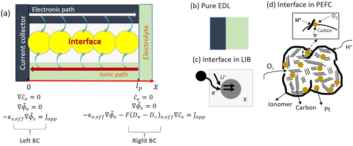
Figure 4. (a) Transmission line representation of electronic and ionic transport in porous electrodes in electrochemical systems and boundary conditions. (b)–(d) Interfaces in supercapacitors, LIBs and PEFCs, respectively.
Download figure:
Standard image High-resolution imageAt  the ion concentration is constant, namely, the perturbation in the ion concentration is zero, and the total current flows through the electrolyte path only, that is
Equations 53, 54 and 55 are put into a concise form,


with the coefficients  expressed as


In what follows,  are taken as constant coefficients. For this end,
  is assumed to be uniform across the porous electrode. It is known that
  is determined by the local concentration of species, potential difference across and structural properties of the EEI. Therefore, the porous electrodes should be homogeneous and there is no concentration or potential gradient under the static state condition (no dc current), in order to justify the assumption of uniform
  In the presence of dc current, numerical solution is usually resorted to.
With algebra manipulations detailed in the SI,  is analytically solved as,
with the coefficient  denoting
and the coefficients 


 are provided in the SI. Though
  is explicitly included in Eq. 64,
  is independent of
  a consequence of linearity of the model, as
 and
and  are proportional to
  and
and  is cancelled out eventually.
The above impedance model can be simplified to a varying extent in following four cases. The first case assumes  or equivalently,
  namely, the electronic conduction is sufficiently fast compared to the ionic transport. This assumption is reasonable in many electrochemical systems, for example, carbon-based/supported electrodes for supercapacitors, LIBs and PEFCs. Under this assumption, we have
 and much simplified expressions for
 The simplified impedance expression for this case 1 is
In the second case, we neglect ionic diffusion in the electrolyte phase. Specifically, Eq. 58 is neglected and Eq. 59 is simplified to

with the corrected expression of ![${{\rm{\Theta }}}_{4}\,=\,\tfrac{{a}_{v}}{{Z}_{loc}}\left[\left(\tfrac{1}{{\kappa }_{e,eff}}+\tfrac{1}{{\kappa }_{s,eff}}\right)\right].$](https://content.cld.iop.org/journals/1945-7111/167/16/166503/revision5/jesabc655ieqn303.gif) Thus, the simplified impedance expression for the case 2 is
Thus, the simplified impedance expression for the case 2 is
with the detailed derivation presented in the SI.
In the third case, we neglect both ionic diffusion and electronic conduction ( a stronger assumption than
  used in the case 1. Therefore, Eq. 68 is further simplified as

which is the standard de Levie model.
In the fourth case, in addition to above assumptions made in the de Levie model, we further assume that  is sufficiently high, satisfying

In this case, the impedance is simply given by

Equation 71 shows that  is proportional to
  with a trivial structural coefficient.
By this point, we have outlined a general theoretical framework of impedance response of uniform porous electrodes impregnated with a symmetric binary electrolyte under the electroneutrality approximation and the static state condition. The theory is expected to be applicable to model impedance response of porous electrodes in supercapacitors, various sorts of metal-ion batteries, and PEFCs. In what follows, we review chronologically literature studies introducing different transport processes and  in the context of the above theoretical framework.
Literature progress: the variety of mass transport and 

The impedance response of gas-diffusion porous electrodes was studied by Darby in 1960s, 88 and by Keddam et al. in 1984. 89 The transport process considered in their models is gas transport in the axial direction, which is coupled to a Faradic reaction, with first- or arbitrary order kinetics, at the pore wall. Double-layer charging current is neglected. The key controlling equation in their models is

where  is the diffusion coefficient and
  a pseudo-homogeneous rate constant. The boundary conditions are:
  at
at  with
with  being the concentration in the solution bulk, and
  at
at  as gas cannot penetrate the pore end. The gas concentration distribution at steady state is obtained as

with  being the thickness of the porous electrode.
When the gas-diffusion porous electrode is submitted to a small perturbing signal around its steady-state condition, the response, namely, the concentration change  can be derived from the Taylor expansion of Eq. 72 limited to first-order terms,

where 
 is a sinuous voltage perturbation, with
  being the amplitude and
  the angular frequency. Via Fourier transform, Eq. 74 is written as

Different from the uniform static-state concentration distribution assumed in the above theoretical framework, Eq. 75 features a nonuniform  given in Eq. 73. For this reason, the model cannot be solved analytically, and numerical impedance simulation is in order.
Lasia extended the de Levie model by replacing  with
with  with
with  being a constant in
  and
and  being the exponent of a constant-phase element (CPE).
90
CPE was firstly proposed by Fricke in 1932 to describe the phenomenon of capacitance dispersion,
91
which may have many possible causes including surface roughness and specific adsorption, see a critical discussion by Pajkossy.
92,93
Brug et al.
94
proposed another CPE expression,
being the exponent of a constant-phase element (CPE).
90
CPE was firstly proposed by Fricke in 1932 to describe the phenomenon of capacitance dispersion,
91
which may have many possible causes including surface roughness and specific adsorption, see a critical discussion by Pajkossy.
92,93
Brug et al.
94
proposed another CPE expression,  where
where  is a constant with the dimension of
  and
and  has the same meaning as
  in Lasia's expression. Zoltowski proposed two definitions of the CPE impedance,
  and
and  95
The dimensions of
95
The dimensions of  and
and  are
are  and
and  respectively. The CPE represents a capacitor for
  a resistor for
  and an inductor for
  Although the CPE expression is different in these models, the transport process is the same as in the de Levie model, namely, ion transport in the electrolyte solution described by the Ohmic law. Replacing the pure capacitance with the CPE gives rise to an inclined tail in low frequency range.
In 1993, Paasch et al. 47 derived the electrochemical impedance based on a macroscopically homogeneous porous electrodes theory. Their model describes ionic conduction in the electrolyte phase and electronic conduction in the solid phase, double layer charging and charge transfer reaction at the solid/liquid interface, and diffusion in the electrolyte-filled pores. They assumed that the electronic conductivity in the solid phase is much larger than the ionic conductivity in the electrolyte phase, so that the solid phase has a uniform electrical potential. The model of Paasch et al. 47 corresponds to the case 1 in the above theoretical framework.
In 1999, Bisquert et al.
96
studied impedance response of a disordered medium with anomalous transport effects that frequently occur in disordered materials where the charge transfer proceeds via discrete transitions between localized states. And they extended the model in the presence of redox reactions in 2000.
97,98
Research in electrical properties of disordered materials has revealed a frequency-dependent ac conductivity  described as

where  is the crossover frequency, and
  For amorphous semiconductors, the values of
  is close to 0.8.
96
The values of
is close to 0.8.
96
The values of  vary widely among different systems and depend on the temperature.
96
Considering this anomalous transport effect,
vary widely among different systems and depend on the temperature.
96
Considering this anomalous transport effect,  is now given by

which shares the same form with  considering the CPE.
In 1999, Eikerling and Kornyshev developed the impedance theory of the catalyst layer of PEFCs based on the macrohomogeneous porous electrode theory.
48
Following mass transport processes are included: (i) proton transport through the polymer-electrolyte porous network, (ii) oxygen supply through hydrophobized gas pores, and (iii) oxygen reduction reaction and double-layer charging at the electrochemical interface. In the case where oxygen transport is neglected, the local impedance is given by,  where the chare transfer resistance is
  with an apparent Tafel slope
  (
( is the number of electrons transferred) and the exchange current density
  The electrode impedance is obtained by substituting
  into Eq. 68 corresponding to the case 2, with the following asymptotic behaviors,
and
When  corresponding to the case 3, above equations are simplified further to

and
Extensions to the Eikerling-Kornyshev impedance model will be reviewed in the section 5.2.
In 2000, Meyers et al. modelled the impedance response for porous electrodes in lithium-ion batteries.
49
As in the de Levie model, the Meyers model describes ion transport in the electrolyte phase and electron transport in the solid phase using the Ohmic law. The model features the expression of  which describes the impedance response of a single intercalation particle, given by

where  is the charge transfer resistance,
  is the equilibrium potential which depends on
  the Li+ concentration in the solid phase.
  is related to spherical diffusion, with
  being the dimensionless frequency-dependent constant,
  the radius of the active particles, and
  the solid-phase diffusion coefficient.
65,99
When
the solid-phase diffusion coefficient.
65,99
When  Eq. 82 is asymptotic to

When  Eq. 82 is asymptotic to

The impedance response of the porous electrode is then obtained by substituting Eqs. 83 and 84 into Eq. 68, corresponding to the case 2. When  the electrode impedance is asymptotic to
And when  the electrode impedance is asymptotic to
Assuming  as in the case 3, Eqs. 85 and 86 can be simplified further as follows,

Impedance models developed for lithium-ion batteries will be reviewed in greater detail in the section 5.1.
Extension in structure
The standard de Levie model
41
assumes an ideally uniform cylinder pore with length  and radius
  that is fully filled with electrolyte solution as depicted in Fig. 2. The corresponding EIS displayed in the Nyquist plot exhibits a 45° line in high frequency range, which is transitioned, in the absence of faradaic reactions, to a strictly vertical line in low frequency range. EIS data measured in real situations deviate from theoretical predictions by showing an arc in high frequency range and/or an inclined line in low frequency range, impelling us to rethink the assumption of a uniform cylinder pore in the de Levie model. This section is devoted to research works in this direction, which are broadly classified into two categories: explicit pores and macroscopic continuum media (referred to implicit pores as the antithesis of explicit pores). Varied explicit pores, including uniform pores, pores with through-plane size distribution, pores with in-plane size distribution, and fractal pores, have been investigated and will be reviewed in this order below. As regards implicit pores, the theoretical formulation is basically the same as presented in the previous section; the vast majority of studies on structural effects concern about gradient design of battery and fuel cell electrodes. Special attention is placed on implicit pores consisting of agglomerates, a common mesoscopic structural element in fuel cell porous electrodes. Please refer to Table III for the list of symbols used in this section.
Table III. List of symbols in section 'Extension in structure'.
| Symbol | Description |
|---|---|

| Length ratio between two adjacent scales in Liu 100 and Kaplan et al. 101 model; |
Side length of the primary pore in Sapoval's model, 
| |

| Cross-section area of pores, 
|

| Capacitance of primary pores, 
|

| Capacitance of outer flat layer, 
|

| Capacitance of elementary species, 
|

| The pore capacitance, 
|

| Fractal dimension |

| Dimensionless shape factor, 
|

| Total current, 
|

| Current through the electrolyte phase of the ith disc, 
|

| Current through the solid phase of the ith disc, 
|

| Scaling factor |

| Total length of the noncylindrical pore, m |

| Length of uniform cylinder pore, m |

| Pore length, 
|

| Transfer matrix of the ith disc |

| Number of discs |

| Mean pore radius of the noncylindrical pore, m |

| Radius of the ith disc, 
|

| Resistance of primary pores, 
|

| Solution resistance out of the pore, 
|

| Specific resistance of the electrolyte phase, 
|

| Resistance of elementary specie, 
|

| Solution resistance out of the pore, 
|

| Specific resistance of the solid phase, 
|

| Solution resistance per unit pore length, 
|

| Pore volume, 
|

| Total pore volume of the electrode, 
|

| Circumference of cross-section of pores, 
|

| Admittance, 
|

| Specific resistance of the interface impedance per unit length, 
|

| Interfacial impedance per unit pore length, 
|

| Area specific interfacial impedance, 
|

| Impedance of the pore, 
|
or total impedance of porous electrode in Eloot's model,
102

| |

| Penetrability |

| Penetrability coefficient |

| CPE exponent |

| Ionic conductivity, 
|

| Penetration depth of the a.c. signal, 
|

| Average deviation of the geometric variable 
|

| The capacitive interface fraction of the pore wall |

| Resistivity of electrolyte, 
|

| Standard deviation of the geometric variable 
|

| Interface potential of the ith disc, V |

| Potential in electrolyte phase, V |

| Potential in solid phase, V |
Explicit pores
Explicit pores have a definite structure, viz., in a specific shape with a definite size, where the solid and electrolyte phases are explicitly separated. In the following, we start with uniform pores, then expand the treatment by introducing through-plane and in-plane distributions, successively, and touch upon fractal pores in the end.
Uniform pore structure
The standard de Levie model expresses the impedance response of a uniform cylinder pore as Eq. 9. Avoiding repeating the standard de Levie model that has been expounded previously, we herein focus on an additional structure effect, firstly pointed out by Lasia et al., concerning the contribution of the outer flat layer, for example, the pore end interfacing the electrolyte, to the total impedance of the porous electrode. 103 This contribution becomes nontrivial in high frequency range where the penetration length is much shorter than the pore length. Under such scenarios, Lasia et al. took into account the capacitance of the top flat layer and modified the impedance response as, 103

where  is the solution resistance out of the pore,
  is the capacitance of outer flat layer and
  is impedance of the pore.
The simulation results (Fig. 5) show an inclined line with a phase angle larger than 45° in high frequency range, in agreement with experiment result (dots in Fig. 5c), and a vertical line in low frequency range. Besides, the phase angle of the inclined line in high frequency range grows as the ratio of the flat capacitance  to the pore capacitance
  increases.
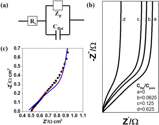
Figure 5. (a) Equivalent electrical circuit of the Lasia model considering the contribution of the outer flat layer to the total impedance of the porous electrode, with  being the solution resistance out of the pore,
  the impedance of the pore,
  the capacitance of the outer flat layer, (b) Nyquist plot with different values of
  and (c) comparison between experiment data (points), the standard de Levie model (solid line), and the Lasia model (dashed line). Subfigure (b) and (c) are reproduced with permission from Lasia et al.
103
and (c) comparison between experiment data (points), the standard de Levie model (solid line), and the Lasia model (dashed line). Subfigure (b) and (c) are reproduced with permission from Lasia et al.
103
Download figure:
Standard image High-resolution imageThrough-plane distribution of pore structure
By through-plane distribution we mean that properties, most often, the pore radius, change along the direction perpendicular to electrode surface. In a pioneering work, Keiser et al.
51
uniformly split the pore into  discs with equivalent height
  but different radius
 each disc is then treated as a uniform cylinder pore with the solution resistance
  and capacitance
  as shown in Fig. 6a.
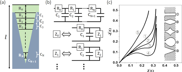
Figure 6. (a) Illustration of a non-uniform pore being divided into N discs (green: electrolyte; grey: solid matrix) and (b) the corresponding transmission line model; (c) the simulated impedance curve in the Nyquist plot of different pores being illustrated in the inset. Subplot (c) is reproduced with permission from Keiser et al. 51
Download figure:
Standard image High-resolution imageAfterwards, considering the solution resistance out of the pore, denoted  the total impedance as illustrated in Fig. 6b is given by

with  determined by the recursion formula,

Dividing both sides of Eq. 91 by  one obtains
where  with
with  (m) being the mean pore radius and
  (m) the total length of the noncylindrical pore,
  is the dimensionless shape factor with
  (
( ) being the radius of the ith disc,
  (
( ) is the penetration depth of the a.c. signal with
 being the ionic conductivity.
Since the pore end is assumed to be insulated  the starting value of the recursion formula reads

The total impedance of the pore can be obtained via iterating Eq. 92 with the initial condition of Eq. 93. With the solution resistance out of the pore being zero ( ), Fig. 6c shows that the pore impedance significantly varies with the pore shape. Even for the case without any Faradaic reaction, a semicircle (usually interpreted as the impedance response of a Faradaic reaction in parallel with double layer charging) is manifested in high frequency range for the pear-shaped pore. Therefore, special care should be added in interpreting a semicircle of impedance curves. Lasia et al. extended the work of Keiser et al. to spherical and bi-spherical pores, and showed that the impedance curve depends on the pore opening size of the spherical pore and two overlapped semicircles exist in the impedance curve of the bi-spherical pore.
104
), Fig. 6c shows that the pore impedance significantly varies with the pore shape. Even for the case without any Faradaic reaction, a semicircle (usually interpreted as the impedance response of a Faradaic reaction in parallel with double layer charging) is manifested in high frequency range for the pear-shaped pore. Therefore, special care should be added in interpreting a semicircle of impedance curves. Lasia et al. extended the work of Keiser et al. to spherical and bi-spherical pores, and showed that the impedance curve depends on the pore opening size of the spherical pore and two overlapped semicircles exist in the impedance curve of the bi-spherical pore.
104
Eloot et al. developed the matrix method to treat through-plane distributions, as shown in Fig. 7.
102
In the matrix method, the pore and the wall material are split up into  discs with random height
  and radius
  (
( ), and each disc is described using the standard transmission line model with constant properties. The current through the electrolyte phase (
 ) and solid phase (
 ) as well as the interface potential (
 ) of the ith disc could be obtained as detailed in SI (S1 ∼ S21). The adjacent discs are correlated by a transfer matrix

where  (
( ) is the total current.

Figure 7. (a) The pore is divided into N discs connected in series and each disc is treated by the standard transmission line model. (b) and (c) are the illustrations of pores with different geometries and the corresponding impedance diagrams simulated using the Eloot et al. model, respectively. Subplot (a)–(c) are reproduced with permission from Eloot et al. 102
Download figure:
Standard image High-resolution imageThe matrix  could be determined by invoking the constraint that the current and potential in both electrolyte and solid phases must be continuous at the interface between two adjacent discs, resulting in
with 


 Here,
Here,  (V) and
  (V) are the potential in electrolyte and solid phases, respectively;
  (
( ),
),  (
( ), and
  (
( ) are the specific resistances of the solid phase, the electrolyte phase, and the interface impedance per unit length, respectively. Provided the transfer matrix, we can determine the total impedance of the porous electrode, defined as,
 ![${Z}_{p}\,=\,[{\varphi }_{s}^{N}-{\varphi }_{e}^{0}]/I,$](https://content.cld.iop.org/journals/1945-7111/167/16/166503/revision5/jesabc655ieqn505.gif) as (the corresponding solving process details are presented Eqs. (S45) to (S67) in the SI),
as (the corresponding solving process details are presented Eqs. (S45) to (S67) in the SI),
Simulated EIS data are displayed in Nyquist plot in Fig. 7c, indicating that the impedance curves depend on the pore shape in high frequency range and converge to vertical lines in low frequency range. In high frequency range, the a.c. signal could only penetrate a part of the pore. Consequently, the total active surface area changes with the frequency and also with the pore shape. This explains why the EIS depends on the pore shape. In low frequency range, the a.c. signal penetrates the whole pore and the total active surface area does not change with the frequency any longer, resulting in an invariably vertical line.
As regards a porous electrode with a capacitive interface and an insulated pore base, Eloot et al. compared the recursion method and the matrix method.
102
The results show that the impedance obtained from the recursion method deviates from a 45° line and does not converge to the origin point of the coordinate system in high frequency range. This is because the recursion method involves serial resistances  which are zero only if
  is infinite. Eloot et al. concluded that the matrix method is more accurate than the recursion method in high frequency range with the same number of discs. In addition, Eloot et al. found that the real part of the impedance obtained from the matrix method depends on the pore geometry, which is in contrast with the results of Keiser et al.
102
Besides the pore shapes mentioned above, de Levie developed V-grooved pores to describe the influence of surface roughness on the electrode impedance.
43
Later on, Gunning obtained an exact solution for the impedance response of the V-grooved pore.
105
is infinite. Eloot et al. concluded that the matrix method is more accurate than the recursion method in high frequency range with the same number of discs. In addition, Eloot et al. found that the real part of the impedance obtained from the matrix method depends on the pore geometry, which is in contrast with the results of Keiser et al.
102
Besides the pore shapes mentioned above, de Levie developed V-grooved pores to describe the influence of surface roughness on the electrode impedance.
43
Later on, Gunning obtained an exact solution for the impedance response of the V-grooved pore.
105
In-plane distribution of pore structure
A porous electrode can be considered as a parallel collection of pores with in-plane distributions of various properties, such as radius, length and so on. Accounting for these in-plane distributions represents a step closer to the reality. Song et al. have pioneered the introduction of pore size distribution into the impedance response of porous electrodes composed of cylinder pores of an identical pore length (Fig. 8). 53,106
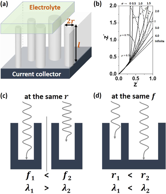
Figure 8. (a) Structural illustration of a porous electrode with a pore size distribution. (b) Impedance response corresponding to a normal distribution with different values of  and
and  (c) Penetration depth (
 ) of the same pore stimulated with different frequencies. (d) Penetration of two pores with different radii stimulated with the same frequency. Subplot (b)–(d) are reproduced with permission from Song et al.
53,106
) of the same pore stimulated with different frequencies. (d) Penetration of two pores with different radii stimulated with the same frequency. Subplot (b)–(d) are reproduced with permission from Song et al.
53,106
Download figure:
Standard image High-resolution imageThe impedance of a single pore given by the de Levie model (Eq. 9) is rearranged in the following form,
where  is a dimensionless impedance, with
  (
( ) being the impedance of a single pore,
  (
( ) the total electrolyte resistance,
  (
( ) the pore length,
  (
( ) the pore radius and
  (
( ) the specific conductance.
  is the penetrability, with
  (
( ) being the penetration depth.
  (
( ) is the penetrability coefficient.
The total impedance of a porous electrode composed of an array of pores in parallel connection is expressed as

where  is a distribution density function of the penetrability coefficient (
 ), Hence,
  means the number of pores between
  and
and 
 is an array of parameters such as, pore size, pore length and so on.
If the structural parameter possessing a distribution is denoted as  one can conduct the transform,
  with
with  given by

Here,  is the pore number between
  and
and  and
and  is the pore volume. Through normalization, Eq. 99 is rewritten as,
 ![$f\left(x:{a}_{2}\right)\,=\,\left[{V}_{tot}/\pi {r}^{2}{l}_{p}\right]k(x:{a}_{2}),$](https://content.cld.iop.org/journals/1945-7111/167/16/166503/revision5/jesabc655ieqn540.gif) with
with  and
and  being the total pore volume of the electrode.
Therefore, the total impedance is given by
Parameterized with a lognormal distribution,  with
with  and
and  being the average and standard deviation of the structural parameter
  which is the pore radius
  in Ref. 53, respectively, Eq. 100 generates synthetic EIS data shown in Fig. 8b. Different from the usual case in Fig. 2, a much more inclined line appears in low frequency when
  is larger, namely, when the pore size distribution is wider. This phenomenon is interpreted as follows. From the expression of the penetration length given by
  it is known that the penetration length becomes longer when the perturbation frequency is lower and when the pore radius is larger. Therefore, when the frequency is high enough that all pores act like a semi-infinite electrode, the overall impedance shows a 45° line. As the frequency decreases, the perturbation length of large pores exceeds the pore length, and the impedance response of these pores transitions to a 90° line, while the overall impedance response of the whole porous electrode shows an inclined line. If the pore distribution is wider, the transition from 45° to 90° lines will extend over a wider frequency range, as shown in Fig. 8b.
Recently, Musiani et al. 107 reconsidered the influence of pore size distribution on the impedance response of a porous electrode. The pore radius r follows a lognormal distribution,
where  with
with  being the median of the pore radius, at which the cumulative probability is 50%, and
  is its standard deviation. And assuming the total pore volume to be half of the electrode (the pore volume fraction was arbitrarily chosen), the number of pores per unit surface is expressed as,

Musiani et al. have calculated the impedance response of the porous electrode with a constant pore volume for two cases: (i) constant median of the pore radius ( ) and variable pore number (
 ); (ii) constant pore number (
 ) and variable median of the pore radius (
 ). In contrast with the work of Song et al., Musiani et al. found the typical 45° line for porous electrode disappeared in high frequency range for the both case.
The main difference between the work of Song et al. and Musiani et al. is that Song et al. adopted pore volume density ( ) while Musiani et al. used pore number density (
 ), to describe the pore distribution. Once a larger standard deviation (
 ) is implanted into the distribution while the total pore volume is constrained, these two different distributions result in disparity. The volume distribution leads to an enormous increase of smaller pore number, thus a decrease of the median of the pore radius, in order to maintain the same total pore volume of pores on each side of the median pore. These smaller pores are accessible at very low frequency and therefore the typical 45° line extends to lower frequencies. In contrast, the pore number distribution retains the same number of pores on each side of the median pore size, which results in a large surface-area ratio of the electrode geometric surface to the pore inner surface when the standard deviation (
 ) becomes larger. As a results, the porous electrode behaves more like a flat electrode and the frequency corresponding to the porous-to-capacitive transition shifts to a higher frequency or even disappears.
Fractal pore structure
A fractal pore possesses similar geometrical patterns at progressively smaller scales. Le Méhauté et al.
108,109
made the first attempt to correlate the fractal dimension  with the CPE exponent,
  as
as

Following the work of Le Méhauté et al., a surge of research activities has sprung up to describe the effect of fractal geometry on the impedance response of interfaces and porous electrodes, among which three representative groups of models are discussed as below.
Liu 100 and Kaplan et al. 101 have independently derived the same formula to describe the relation between the fractal dimension and the CPE exponent in low frequency range. The fractal interface is pictured as a hierarchical network, as depicted in Fig. 9b, in which a portion of the pore at the upper scale is split into two branches at the lower scale with a scaling length ratio of a. The impedance of this hierarchical network is mapped into an equivalent electrical circuit depicted in Fig. 9a, of which the impedance is expressed as,
where  is the length ratio between two adjacent scales;
  and
and  are the resistance and capacitance of primary pores, respectively. Substituting
  with
with  in Eq. 104 and multiplying the fraction by
  yield
yield


Figure 9. (a) The equivalent electrical circuit and (b) the schematic illustration of the pore structure treated in the Liu model, 100 (c) the numerically simulated impedance of the Liu model, 100 (d) the equivalent electrical circuit of the Pajkossy et al. model. 110 Subplot (a)–(d) are reproduced with permission from the corresponding works.
Download figure:
Standard image High-resolution imageAssuming that  diverges much slower than
  namely,
  goes to 0, as
  the low-frequency limit of Eq. 105 becomes
  (the ohmic resistance R has been safely neglected). Then, the recursion expression of the impedance response is given by

with,

where 
 and
and  are the scaling factor, the CPE exponent and the fractal dimension of the interface, respectively. When
  the fractal dimension of the interface converges to zero. In other words, when the interface is an ordinary smooth interface, we retrieve the classical result of
As for a finite number of generation of new branches, numerical calculation in Fig. 9c shows a frequency-independent regime in low frequency range and a frequency-dispersion regime in intermediate frequency range. Specifically, the frequency-dispersion regime is extended to lower frequencies for the interface with a larger number of generation of branches. This is because a larger generation number stands for a rougher interface with more small and deep pores, which are penetrated only by lower frequency signals.
Pajkossy et al.
110,111
recognized that a practical electrode may contain many kinds of self-similar irregularities, such as grooves, cracks, pores and so on, and can be described, approximately and without going into the detailed irregularities, as self-similar fractals with an effective dimension ( ). By dividing the electrode into elementary pieces in parallel connection (Fig. 9c), Pajkossy et al. express the admittance of the electrode as

where  and
and  are the capacitance and resistance of elementary species, respectively.
The admittance  is a two-dimensional macroscopic quantity, which should be inversely correlated with the macroscopic surface area. The capacitance
  a microscopic quantity, should be proportional to the microscopic surface area. The resistance
  is of bulk nature which is inversely proportional to the scale of the object. Consequently, the following scaling laws are obtained when scaling up the macroscopically two-dimensional electrode by a factor of
where 1 stands for the original system and  the newly enlarged system.
Hence, the admittance of the new system is given by
which is transformed to
We have for the CPE,  which gives the relationship
  Equation 111 describes a CPE with an exponent,

For a smooth surface  this correlation gives
  as expected.
Fractal models introduced above treat a rough interface, rather than a porous electrode (a porous electrode has deep pores while a rough interface has shallow pores). Sapoval constructed a porous electrode model by combining the transmission line model and the fractal model as shown in Fig. 10b.
112,113
The porous electrode is pictured as N square holes with the side length reduced by a factor  at the surroundings of the primary pore and the corresponding fractal dimension is then calculated as

with 

Figure 10. (a) Equivalent electrical circuit and (b) the schematic illustration of the pore structure treated in the Sapoval model. 112 (c) The equivalent electrical circuit and (d) the schematic illustration of the pore structure treated in the and Itagaki et al. model. 114 Subplot (b)–(d) are reproduced with permission from the corresponding works.
Download figure:
Standard image High-resolution imageEach pore is described using the de Levie method. The admittance of a pore obtained at nth stage of the decimation is given by
where  is the side length of the primary pore,
  is the capacitance per unit area, l is the pore length,
  is the electrolyte conductance. Accordingly, the total impedance of the electrode is

which converges when N
 meaning that the highest fractal dimension that can be described by this model is
In case of  the total impedance is dominated by small pores, the impedance thus diverges. In case of
  there is no explicit equation to correlate the fractal dimension and the exponent of CPE, but numerical results of Eq. 115 exhibits frequency dispersion in low frequency range, with a CPE exponent that is same as the value in the Liu model.
100
there is no explicit equation to correlate the fractal dimension and the exponent of CPE, but numerical results of Eq. 115 exhibits frequency dispersion in low frequency range, with a CPE exponent that is same as the value in the Liu model.
100
Itagaki et al. 115,114 have modelled a fractal structure with a three-scale pore structure (macropores, mesopores and micropores). The pores at the lower scale randomly locate on the pore wall at the upper scale as shown in Fig. 10d. Following the de Levie model, the impedance of a triangular pore is given by,

with  and
and  Here,
Here,  (
( ) is the solution resistance per unit pore length;
  (
( ) is the area specific interfacial impedance;
  is the resistivity of electrolyte (
 );
);  (
( ) is the pore length;
  (
( ) is the interfacial impedance per unit pore length;
  (
( ) is the cross-section area of pores;
  (
( ) is the circumference of cross-section of pores; and the subscript
  stands for macropores, mesopores and micropores, respectively.
There are  micropores per unit area of the mesopore wall. (1−
 ) of the mesopore wall is occupied by these micropores, and the remaining part with a fraction of
  by the capacitive interface. Therefore, the mesopore impedance is expressed as,
In the same way, the macropore impedance is derived from the mesopore impedance via,

where  is the number of mesopores per unit area of the macropore wall.
Provided with the scaling coefficient  for the pore depth and side length, the total impedance of the porous electrode is readily simulated using Eq. 119. The typical impedance spectra simulated using the model of Itagaki et al. exhibits a frequency dispersion region in high frequency range and a vertical line in low frequency range. If there is no mesopore on the macropore wall (
 ), the impedance response exhibits a 45° line in high frequency range, regressing to the standard behavior of the de Levie model. If the pore wall at the upper scale is totally occupied by sub-pores, the impedance response exhibit 22.5° and 11.25° lines in high frequency range for the double- and triple-scale pore structure, respectively. As
  decreases from 1 to 0, the typical 45° line in high frequency range decreases to a 11.25° line, indicating that less capacitive interface is detected by the a. c. signal. This is because the pore wall with a lower
  is dominated by more small pores on the upper scale, which can be penetrated only at much lower frequency. Readers are also referred to Lasia's book
15
for a comprehensive account of experimental and modelling works on fractals.
is dominated by more small pores on the upper scale, which can be penetrated only at much lower frequency. Readers are also referred to Lasia's book
15
for a comprehensive account of experimental and modelling works on fractals.
Implicit pores: macrohomogenous porous electrode theory
The explicit pore approach may be inadequate for a porous electrode with a large variety of pore structure. In such circumstances, the macrohomogenous porous electrode theory based on the volume averaging method is useful.
4,6,40
In this implicit pore approach, the structure complexity is largely reduced by using average structural parameters, such as the void volume fraction ( ). Effective transport properties are used to reflect the impact of the porous structure on mass and charge transport, as expressed in Eqs. 50–52.
In macrohomogenous porous electrode theory, a widely studied structural effect is so-called gradient design for batteries and fuel cells. As for fuel cells, it have been found that 1) in the gas diffusion layer (GDL), increasing the porosity and PTFE content (hydrophobicity) from the catalyst layer (CL)/GDL interface toward the GDL/channel interface along the through-plane direction and from the channel inlet to the outlet in the in-plane direction improve the cell performance at high current densities 116–126 ; 2) in the micro porous layer (MPL), increasing the PTFE content from the CL∣MPL interface to the MPL∣GDL interface helps to hydrate the membrane under low humidity and to remove liquid water from the electrode under high humidity condition 127 ; 3) in the CL, a decrease in the ionomer content from the membrane/CL interface to the CL/GDL interface benefits the cell performance. 128,129
There has also been a surge of interest in gradient design for LIBs, but controversial conclusions exist. For instance, the gradient porosity distribution designed by Subramanian et al. 130,131 decreases from the separator to the current collector in the cathode electrode, which agrees with the conclusion of Maute et al. 132 On the contrary, Srinivasan et al. 133 and Hosseinzadeh et al. 134 show that the gradient porosity distribution leads to marginal improvement of the cell performance as compared with the uniform counterpart. However, these works did not discuss the impedance response, which can be readily calculated using the methods developed for nonuniform explicit pores.
An interesting structural effect frequently encountered in macrohomogenous porous electrode theory is agglomeration. An agglomerate is formed by holding together a group of particles on a smaller scale. As shown in Fig. 11, the agglomerate (∼200 nm) in fuel cell electrodes is composed of carbon black particles (∼20 nm) deposited with platinum nanoparticles. 135 Intra-agglomerate mesopores (2 ∼ 20 nm) are partially penetrated with ionomer. In addition, the surface of the agglomerate is partially covered with an ionomer film. The oxygen dissolves into the ionomer thin film covering the surface of the agglomerate and then undergoes reaction-coupled diffusion inside the agglomerate.
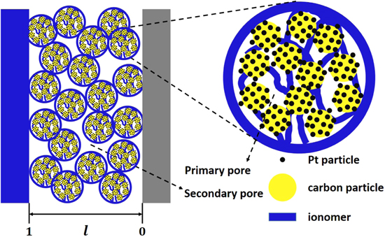
Figure 11. Illustration of a porous fuel cell electrode consisting of agglomerates covered with ionomer on the outmost surface.
Download figure:
Standard image High-resolution imageGerteisen et al. modelled the case where ionomer cannot impregnate the inner pores of the agglomerate and therefore ORR does not occur on platinum nanoparticles inside the agglomerate due to the lacking of protons. 74 In general cases where the ORR occurs inside the agglomerate, the agglomerate per se is a spherical porous electrode with ORR-coupled oxygen and charge transport. Consequently, the whole porous electrode actually possesses a three-scale structure, including the solid-electrolyte interphase (with Debye length as the characteristic length) where the ORR occurs at the bottom of the scale spectrum, the agglomerate scale, and the electrode scale. More impedance models of PEFC will be introduced in section 'Polymer electrolyte fuel cells'. The same circumstance is encountered in LIBs. Huang et al. have developed a three-scale impedance model for LIB electrodes, 65,66 which will be introduced in section 'Batteries'.
Extension in order
In the strict sense of the term, EIS is a linear analysis method. To ensure the linearity in EIS measurements, a small perturbation is applied to the electrochemical system, and the impedance response at the same frequency as that of the perturbation is subject to analysis, namely, fundamental-order impedance analysis is carried out. This way, substantial information of system hidden in high-order impedance would be missed out. Hence, there is a clear need to obtain higher-order impedance and to extend EIS from linear to nonlinear regime. There have been continued efforts in this direction, as summarized in a recent review article. 58 A somewhat paradoxical terminology, nonlinear electrochemical impedance spectroscopy (NLEIS), has emerged from these studies. NLEIS measurements, with a large alternating perturbation applied to the system under investigation, enhance the signal-to-noise ratio and permit high-order impedance analysis. Please refer to Table IV for the list of symbols used in this section.
Table IV. List of symbols in section 'Extension in order'.
| Symbol | Description | Value |
|---|---|---|

| Double-layer capacitance | Eq. 140 |

| First-order double-layer capacitance | Eq. 145 |

| Second-order double-layer capacitance | Eq. 146 |

| Gouy-Chapman capacitance | Eq. 142 |

| Helmholtz capacitance | Eq. 141 |

| Concentration of metal ions | Eq. 122 |

| Bulk concentration of metal ions |

|

| Diffusion coefficient |

|

| Elementary charge |

|

| Equilibrium voltage |

|

| Frequency |

|

| Perturbation magnitude |

|

| Sinusoidal voltage signal |

|

| Faraday constant | 96485 
|

| Exchange current density |

|

| Faradaic current density | Eq. 121 |

| Boltzmann's constant |
|

| Avogadro's number |

|

| Ideal gas constant | 8.314 
|

| First-order charge-transfer resistance |

|

| Effective second-order charge-transfer resistance | Eq. 150 |

| Temperature | 298.15 
|

| Distance from electrode surface to bulk solution | 0.01 m |

| First-order impedance | Eq. 147 |

| Second-order impedance | Eq. 148 |

| Charge transfer coefficient |

|

| Vacuum permittivity |
|

| Permittivity of bulk water |

|
| η | Overpotential |

|

| Debye length |

|

| First-order mass transfer coefficient |

|

| Second-order mass transfer coefficient |

|

| Angular frequency |

|
Although there have been considerable interests in measuring the NLEIS of porous electrodes in electrochemical systems, as reviewed by Fasmin and Srinivasan 58 in 2017, theoretical and modelling efforts are yet sparse. Of note, Murbach and Schwartz 59 numerically calculated the high-order impedance response of battery porous electrodes based on the Newman model. Their simulation has demonstrated that the second-order impedance, compared with fundamental-order impedance, shows stronger dependence on the charge transfer coefficient, and the derivative of open circuit potential with respect to lithium ion concentration in certain frequency range.
A theory of NLEIS of porous electrodes is, to the best knowledge of the authors, missing yet. Nevertheless, the theory of NLEIS of an electrochemical interface has been developed by Wong and MacFarlane 62 in 1995. Wong and MacFarlane considered charge transfer reactions, both reversible and irreversible, and mass transfer, while the double-layer charging process was neglected in their treatment. In what follows, for the purpose of grasping basic principles of NLEIS, we set out to derive the NLEIS of an electrochemical interface. Our derivation closely follows the route paved by Wong and MacFarlane and extends the Wong-MacFarlane theory by including the double-layer charging process. General features of second-order impedance response of an electrochemical interface are discussed using the model.
Let us consider a general electrochemical interface, as schematically shown in Fig. 12, where double-layer charging and diffusion-coupled faradaic reactions occur. The electrolyte is symmetric and monovalent. In our treatment, the double-layer charging process is described using Gouy-Chapman-Stern (GCS) model, the diffusion process using Fick's law, and the Faradaic reaction using Butler-Volmer theory. The electrochemical interface is perturbed by a sinusoidal voltage signal,  with
with  being the difference between the equilibrium potential of the reaction and potential of zero charge, and
  the perturbation magnitude. The overarching task is to calculate the current response at a series of orders. Combining the voltage perturbation and current response, we can calculate the impedance response at the same series of orders.

Figure 12. Schematic illustration of an electrode-electrolyte interface with metal deposition reaction occurring at the interface.
Download figure:
Standard image High-resolution imageAt the electrode-electrolyte interface (EEI),  the following redox reaction takes place,

where  denotes the metal ion and
  the metal atom. According to the Butler-Volmer equation, the reaction current density reads
136
the metal atom. According to the Butler-Volmer equation, the reaction current density reads
136

where η is the overpotential, 
 the charge transfer coefficient,
  the exchange current density,
  the concentration of metal ions at the electrode surface,
  the bulk concentration of metal ions, and other symbols have their usual meanings. In order to calculate
  using Eq. 121, we need to solve the time-dependent concentration,
  which is determined from

where  denotes the diffusion coefficient. We have neglected migration in Eq. 122. Equation 122 is closed with initial and boundary conditions detailed below.
Initially, the concentration has its bulk value,

At the EEI,  the flux of the metal ion is related to the reaction current density via

In the bulk solution,  metal ion has its bulk concentration,

Solving Eq. 122 with the initial and boundary condition yields (we refer readers to the SI for a detailed derivation),
Substituting Eq. 126 into Eq. 121, expanding the exponential terms into Taylor series, and then equating the coefficients of equal power of  yield
62
yield
62
where 
 and
and 
At the order of  Eq. 127 is simplified as

which leads to

in the frequency domain. Consequently, we have  which is trivially the mathematical representation of the stationary condition.
Similarly, when  Eq. 127 gives
Given that  and using the relation
  Eq. 130 is reduced to

Transforming Eq. 131 into the frequency domain, we have

where  Then, using the relationship
  and concentrating on the first-order term yield,

where  is the charge-transfer resistance, and
  is the mass transfer coefficient.
When  Eq. 127 is written as
Substituting Eq. 129 into Eq. 134 and using the identity  we have
Herein,  is calculated from Eq. 132 by means of inverse Laplace transform,
where  denotes inverse Laplace transform. Now substituting Eq. 136 into Eq. 135 and using the identity
  we obtain
We now embark on transforming trigonometric terms into potentials of different orders. We define a second-order potential,  Then we have,
  and
and  with
with  being the Laplace-transform operator and
  the Laplace-transformed counterpart of
  As
As  we have,
  Treatment of
  is troublesome, and we make the following approximation, inherited from Wong and MacFarlane,
62
of
is troublesome, and we make the following approximation, inherited from Wong and MacFarlane,
62
of  Afterwards, neglecting the
  terms, and transforming Eq. 137 into the frequency domain, we obtain
Using the relation  we have the second-order Faradaic current density,

By this point, we have obtained the first- and second-order Faradaic current densities. We now turn to double-layer charging process, which is widely described using GCS model,

where  denotes the Helmholtz capacitance and
  the Gouy-Chapman capacitance, expressed, respectively, as

and

where  is the thickness of the Stern layer,
  the relative dielectric permittivity of solvent and
  the dielectric permittivity of vacuum, and
  the Debye length,
  Substituting Eqs. 141 and 142 into Eq. 140 yields,

The double-layer charging current density is calculated as

Transforming Eq. 144 into the frequency domain, expanding the exponential term into Taylor series, and using first-order terms, we have
where  is the ordinary double-layer capacitance. Similarly, expanding the exponential term into Taylor series and using second-order terms yield,
where  is the second-order double-layer capacitance.
The total current density is the sum of Faradaic and double-layer charging parts, viz.,  with
with  indexing the order. The nth-order interfacial impedance is defined as
  Hence, combining Eqs. 133 and 145, we obtain the first-order impedance,

Similarly, combining Eqs. 139 and 146, we obtain the second-order impedance,
Figure 13 shows the first- and second-order impedance plots with model parameters listed in the figure caption. Analytical results calculated using Eqs. 147 and 148 are compared with numerical results which are obtained by numerical Fourier transform of the total current density simulated using Eqs. 121, 122 and 144 with corresponding boundary conditions. Notably, numerical and analytical results agree on the first-order impedance, which is composed of a straight line in low frequency region and a semi-circle in high frequency region. As for the second-order impedance, the analytical expression captures overall feature of the numerical results, but the two deviate noticeably. The deviation originates from the approximation made in treating the  term in Eq. 137. Circumventing this approximation leaves as a task for future investigation. Compared to the first-order impedance, the second-order impedance displays distinct graphical characteristics. Most notably, the second-order impedance is composed of an arc in high-mediate frequency range and an inclined line in low frequency range. In addition, the arc in high-mediate frequency range depends strongly on the charge transfer coefficient. Asymptotic analysis to Eq. 148 provides deeper insights into the graphical features.
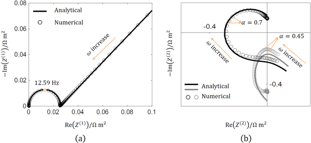
Figure 13. (a) Nyquist plot of the first-order impedance,  (b) Nyquist plot of the second-order impedance,
  Model parameters are:


Download figure:
Standard image High-resolution imageIn the high frequency limit, namely,  Eq. 148 is simplified to

where the effective charge transfer resistance and double-layer capacitance are given by
with  When
When  and
and  are constant, Eq. 149 represents a semicircle in Nyquist plot. Both
  and
and  depends on frequency, however, leading to a nearly full arc in Nyquist plot. The real and imaginary parts of Eq. 149 are
  and
and  respectively. When
  varies from 0.3 to 0.7,
  is always less than zero. When
 and the impedance response of Eq. 149 locates in the second quadrant of Nyquist plot. When
 and the impedance response of Eq. 149 locates in the third quadrant of Nyquist plot. As for the behavior of the second-order impedance in low frequency limit, namely, when
  Eq. 148 is asymptotic to

where  is the second-order mass transfer coefficient. It is readily seen that Eq. 152 manifests itself as a 45° line in Nyquist plot, as in the first-order impedance.
Selected Applications
Batteries
There are usually four scales in a battery porous electrode, as depicted in Fig. 14. On the topmost scale, the electrode has a complex porous structure with a thickness on the order of hundreds of microns. On the second scale, agglomerates with a radius of several microns are found. Further zooming in, one sees primary particles with a characteristic size of tens to hundreds of nanometers. On the bottom scale, there is usually a compact solid-electrolyte interphase (SEI) with a thickness of several nanometers on the surface of primary particles. There has been continued efforts to model the impedance response of lithium-ion batteries, either focusing on one scale or extending over multiple scales. In the following, we first present a theoretical analysis for each of these scales in a bottom-up order, setting the stage for reviewing the theoretical progress on this topic. Afterwards, selected examples of applications of EIS in battery research are introduced. For the sake of completeness, the newly developed impedance model of the SEI is included. Please refer to Table V for the list of symbols used in this section.

Figure 14. Four scales in a battery electrode.
Download figure:
Standard image High-resolution imageTable V. List of symbols in section 'Batteries'.
| Symbol | Description |
|---|---|

| Concentration of Li+, 
|

| Capacitance of the compact layer, 
|

| Double layer capacitance of the compact layer, 
|

| Double layer capacitance of the porous layer, 
|

| Total double layer capacitance of the compact-porous interface, 
|

| Tracer diffusion coefficient, 
|

| Chemical diffusion coefficient, 
|

| Ambipolar diffusion coefficient, 
|

| Differential diffusion coefficient, 
|

| Diffusion coefficient of primary particles, 
|

| Equilibrium potential, 
|

| Standard equilibrium potential, 
|

| Coefficient in Eq. 157 |


| Coefficients in Eq. 160 |

| Exchange current density, 
|

| Applied current density, 
|

| Exchange current density corrected with double layer effects, 
|

| Double layer charging current density, 
|

| Faradaic current density, 
|

| Radius of agglomerates, 
|

| Resistance of charge transport across the compact layer, 
|

| Charge transfer resistance of primary particles, 
|

| Ion-transfer resistance, 
|

| Radius of primary particles, 
|

| Open circuit potential, 
|

| Frequency-dependent factor of spherical diffusion, 
|

| Impedance of agglomerates, 
|

| Impedance at the compact-porous interface, 
|

| Diffusion impedance of primary particles, 
|

| Impedance of primary particles without SEI film in Eq. 178/with SEI film in Eq. 180, 
|

| Impedance of the SEI, 
|

| Activity coefficient |

| Dimensionless length coefficient in Eq. 167 |

| Coefficient embodying the effect of ion transport on the ion transfer reaction |

| Ionic conductivity, 
|

| Characteristic length of diffusion in bulk electrolyte, 
|

| Characteristic length of diffusion in the porous layer, 
|

| Distance between the reaction plane and electrode surface, 
|

| Electrolyte phase volume fraction of agglomerates |

| Porosity of the porous layer |

| Overpotential, 
|

| Frequency-dependent dimensionless parameter |

| Tortuosity of agglomerates |

| Time constant of solid phase diffusion, s |

| Structure parameter of primary particles |
Solid electrolyte interphase
The SEI film has a bilayer structure consisting of an inner compact layer and an outer porous layer.
137–139
As shown in Fig. 15,  locates the electrode surface,
  ("c" stands for "compact") the compact layer,
  ("p" stands for "porous") the porous layer,
  the bulk electrolyte, and
  ("e" stands for "electrolyte") the mid-plane of the bulk electrolyte phase with
  being the thickness of the electrolyte bulk. It is safe to draw the approximation of
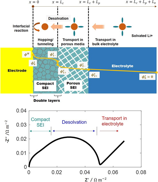
Figure 15. Bilayer structure and physio-chemical processes of the SEI at a lithium metal anode and the simulated EIS based on Eq. 177 using the following parameters: 


Download figure:
Standard image High-resolution imageThe porous layer is impregnated with an electrolyte solution, allowing electrolyte-phase transport of solvated Li+ and anions. At the compact-porous interface,  Li+ ions have to undergo desolvation, which is proposed to be the rate-determining step by Ogumi.
140–142
Secondary ion mass spectrometer analysis from Lu and Harris leads us to assume that anions cannot penetrate through this interface.
143
In the compact layer, there may be multiple charge carriers, among which we assume excess interstitial Li+ ions are the major player. At the interface between the electrode and the compact layer,
Li+ ions have to undergo desolvation, which is proposed to be the rate-determining step by Ogumi.
140–142
Secondary ion mass spectrometer analysis from Lu and Harris leads us to assume that anions cannot penetrate through this interface.
143
In the compact layer, there may be multiple charge carriers, among which we assume excess interstitial Li+ ions are the major player. At the interface between the electrode and the compact layer,  Li+ ions intercalate into the electrode structure or capture an electron and deposit on the electrode surface. Electrical double layers are formed at the interface between the active particle and the compact layer, as well as the interface between the compact layer and the porous layer. There is no double-layer effect between the porous layer and the bulk electrolyte as ion transport occurs in the same electrolyte phase. In the literature, the relation between the electrical double layer and the SEI film is sometimes obscure and even confusing. Here, we note that the SEI film is a phase and the electrical double layer exsits between two phases.
As the thickness of the bulk electrolyte is usually several orders larger than the Debye length (ca. 0.1 nm for 1M electrolyte), the electroneutrality condition, implying that the concentration of Li+ is equal to that of anions, both denoted as  is satisfied. In bulk electrolyte, Li+ transport via diffusion and migration, which are described by the Nernst-Planck equation in the frequency domain (a phenomenological free energy based derivation can be found in Ref. 99),


where the variables  and
and  are perturbed concentration and potential that are zero at steady state. Here
  is the ambipolar diffusion coefficient, and
  and
and  are the chemical diffusion coefficient and the tracer diffusion coefficient in the dilute-solution limit, respectively, which are correlated as
  with
with  being the activity coefficient.
  is the differential diffusion coefficient.
  is the ionic conductivity.
At the midplane of the bulk electrolyte,  a symmetric condition applies,

At the boundary between the porous layer and the bulk electrolyte,  the concentration and its gradient should be continuous,

where  and
and  are to be derived from the submodel of the porous layer. The subscript "2−" denotes the compact-layer side of the interface at
  The subscript "2+" denotes the bulk-electrolyte side of the interface at
Solving Eq. 153 in the frequency domain with the boundary conditions in Eq. 155 and applying the approximation that  result in,

with  being the characteristic length of diffusion in bulk electrolyte, and
  a coefficient to be determined later.
Ion transport in the porous layer is essentially the same as in the bulk electrolyte; the only difference is that the transport parameters should be replaced with effective values considering the effect of the porous structure,


where  is the porosity of the porous layer,
  and
and  are the effective ambipolar and chemical diffusion coefficient in the porous layer, respectively, and
  is the effective ionic conductivity.
The solution to Eq. 158 is given by
with  being the characteristic length of diffusion in the porous layer.
  and
and  are two coefficients to be determined by the boundary conditions. At the interface between the bulk electrolyte and the porous layer,
  the continuity conditions expressed in Eq. 156 apply. At the compact-porous interface,
  the current flux is carried by cations only and the flux of anions is zero, as a result,
99
the current flux is carried by cations only and the flux of anions is zero, as a result,
99

with  being the applied current density. Applying the boundary conditions, we obtain
with  being a frequency-dependent dimensionless parameter.
Provided the concentration distribution, we are to calculate the potential distribution. The current densities in the electrolyte solution and the porous layer are given by


Integrating Eqs. 164 and 165 and substituting concentration distribution, we solve the potential drop in the porous layer and bulk electrolyte, from which we arrive at the expression for the impedance corresponding to Li+ transport in the bulk solution and the porous layer,

with  being a dimensionless length coefficient related to ion transport, defined as
In Eq. 166, the term  corresponds to migration in half of the bulk electrolyte, the term
  migration in the porous layer, and the term
  diffusion in the porous layer and the bulk electrolyte.
At the compact-porous interface,  a solvated
  ion in solution,
  undergoes desolvation and then hops into the solid phase,

with  being coordinate number of solvents. This ion transfer reaction can be described using the Butler-Volmer equation,
where  is the exchange current density, which is dictated by the activation energy of the desolvation process, and
  the overpotential with
  being the equilibrium potential.
  where
where  is the standard value,
  and
and  are taken at the diffuse-diffusion boundary. The subscript "1-" and "1+" denote the compact-layer and porous-layer side of the interface at
  respectively, as shown in Fig. 15.
Under a small perturbation, Eq. 169 is written as

where  denotes the concentration at the steady state. Here, we neglect variations in
  exerted by the perturbation, for the fact that the compact layer is very thin, and the concentration in the compact layer is controlled by double layer effects.
In addition to the Faradaic current contributed by the ion transfer reaction, there is also double layer charging current at the interface between the compact layer and the porous layer. Since the compact layer is a semiconductor, the double layer is composed of two parts in series, a part belonging to the solution phase, and a part to the solid phase.
144
As a result, the total double layer capacitance,  is thus given by

where  and
and  refer to the double layer capacitance of the compact and porous layer, respectively. No attempt is made, herein, to relate
  and
and  with physical properties of the compact and porous layer, because such practice involves many parameters at the microscopic scale of the interface that are difficult to obtain at the present.
The total current density is the sum of two parts: Faradaic and double layer charging, namely,

with the double layer charging current density given by

Substituting Eqs. 170 and 173 into Eq. 172 with some mathematic manipulations, we obtain the impedance at the compact-porous interface as

with  being the ion-transfer resistance, and
  embodying the effect of ion transport on the ion transfer reaction.
Next, we model the compact layer as a like solid electrolyte with only one ion moving, namely, composed of mobile Li+ in a rigid neutralizing background of negative charge. Li+ transport in the compact layer can be described using the PNP equation. Jamnik and Maier are able to convert the PNP equation into an equivalent circuit representation.
145,146
Further neglect of spatial variation of circuit elements, which is valid beyond the diffuse layer, leads them to obtain analytical impedance expressions.
145,146
However, the compact layer in our case, whose thickness is comparable with the Debye length, is governed by the double layer effects, and the assumption used in the model of Jamnik and Maier to obtain analytical results is invalid any longer. Nevertheless, the model of Jamnik and Maier reveals an important observation that the impedance of the compact layer manifests itself as a semicircle in the high-frequency range. Consequently, we employ a phenomenological model for the compact layer for the moment, which is a parallel connection of a capacitance,  and a resistance related with charge transport across the compact layer,
  namely,

We are left with the task of relating the capacitance and the charge transport resistance with physical properties of the compact layer. This task is by no means trivial. The complexities are two-fold, to say the least. Regarding  it is a mixed capacitance composed of the differential double layer capacitance, the dielectric capacitance, and the chemical capacitance. These three types of capacitance are connected in a complex circuit, rendering a closer examination of
  challenging for the moment. Regarding
  we could express it as

with  being the effective conductivity of the compact layer. By effective we mean it is an overall quantity as the charge conductivity is spatially dependent, an immediate consequence of the distribution of the concentration of charge carriers, in the compact layer.
Combined, we express the impedance of the SEI shown in Fig. 15 as follows,
where the first, second and third term on the right-hand side denotes the impedance of solid-state ion transport in the compact layer, ion desolvation at the compact-porous layer interface, and electrolyte-phase ion transport in the porous layer and the solution bulk, respectively. Note that the charge transfer reaction at the electrode-compact layer interface is not included in  but will be included in the impedance of primary particles. Assigning model parameters with typical values as listed in the caption of Fig. 15, we simulate the EIS as shown in Fig. 15. In the Nyquist plot, we see a high-frequency semicircle corresponding to solid-state ion transport via the compact layer, a moderate-frequency semicircle corresponding to desolvation of Li+ ions at the compact-porous layer interface, and a 45° line in low-frequency range corresponding to transport of Li+ ions through the porous layer and the solution bulk.
Primary particle
A primary particle may have a SEI film covered on its surface or be bare without a SEI film. Huang et al. have developed an impedance model for a spherical primary particle without a SEI film, considering the complex coupling between intercalation and deintercalation of lithium ions at the interface, double-layer charging, and diffusion in solid phase. 65 The impedance expression for the case without a SEI film is given by

where  is a structural parameter with
  being the distance between the reaction plane (assigned as the outer Helmholtz plane in Ref. 65) and the electrode surface, and
  being the Debye length of the double layer of the primary particle.
  is the double layer capacitance at the electrode-electrolyte interface.
  is the charge transfer resistance with
  being the exchange current density corrected with double layer effects,
  is the diffusion impedance with
  being the local slope of the open circuit potential (U) curve as a function of the lithium ion concentration in solid (
 ),
),  being a frequency-dependent factor of spherical diffusion,
147,148
being a frequency-dependent factor of spherical diffusion,
147,148

Here  is the time constant of solid phase diffusion with
  being the radius and
  the diffusion coefficient. It is worth noting that the diffusion impedance is in a form different with the oft-used Warburg impedance based on semi-infinite planar diffusion. Recently, Huang extended the diffusion impedance to different structures with different boundary conditions.
99
the diffusion coefficient. It is worth noting that the diffusion impedance is in a form different with the oft-used Warburg impedance based on semi-infinite planar diffusion. Recently, Huang extended the diffusion impedance to different structures with different boundary conditions.
99
Manifestation of double layer effects in Eq. 179 is two-fold. On the one hand, the exchange current density is corrected with double layer effects, namely,  with
with  being the potential drop in the diffuse layer and
  the symmetry factor. On the other hand,
  is introduced to consider the double layer structure on the charge transfer reaction.
As regards primary particles covered by a SEI film, we combine Eqs. 177 and 178 and obtain the following impedance expression, 65
In Eq. 180, we have neglected  corresponding to ion transport in the bulk electrolyte phase, which will be considered on a higher scale. In addition, we have divided the interfacial charge transfer reaction into three steps: desolvation at the compact-porous layer, ion transport in the compact layer, and electron transfer at the electrode-compact layer interface, corresponding to the third, second, and first term on the right hand, respectively. The division brings many parameters which are unfortunately difficult, if not impossible, to obtain from impedance measurement on a cell. Model systems are required to determine them, instead.
Agglomerate
An agglomerate (secondary particles impregnated with electrolyte) consisting of primary particles is actually a spherical porous electrode. Huang et al. developed a physical impedance model for a spherical agglomerate, starting with deriving basic equations of mass transport from a general free energy functional, continuing with applying the volume averaging method to describe mass transport in porous media, and ending with employing Fourier transform to solve the impedance response. 65 An analytical impedance expression is obtained

with  Here,
Here, 
 and
and  are the radius, electrolyte phase volume fraction and tortuosity of the agglomerate, respectively.
  is the electrolyte conductivity in the agglomerate.
  is difference diffusion coefficient.

 and
and  are functions of matrix elements Θi
 as expressed in Eqs. 60–63. The matrix elements Θi
are functions of properties of primary particles, as given by Eq. (A3.3) in Ref. 65.
as expressed in Eqs. 60–63. The matrix elements Θi
are functions of properties of primary particles, as given by Eq. (A3.3) in Ref. 65.
The impedance response of agglomerates can be measured using the single particle technique. Figure 16a compares the model simulation and the EIS data measured by Dokko et al. on a LiCoO2 particle with a diameter of  at different storage time.
149
The measured EIS data show a 45° line in the high frequency range, a clear fingerprint of porous electrodes, indicating that the single particle composed of primary particles has pores impregnated with electrolyte. The model expressed in Eq. 181 well captures this feature. On the contrary, the model neglecting electrolyte transport inside the single particle does not agree, qualitatively, with experimental data in high frequency range. In addition, the Warburg impedance cannot fit the impedance data in low frequency because solid diffusion in primary particles takes place in a spherical structure rather than the semi-infinite structure assumed in the Warburg model. However, the model expressed in Eq. 181 agrees well with the experimental data also in low frequency.
at different storage time.
149
The measured EIS data show a 45° line in the high frequency range, a clear fingerprint of porous electrodes, indicating that the single particle composed of primary particles has pores impregnated with electrolyte. The model expressed in Eq. 181 well captures this feature. On the contrary, the model neglecting electrolyte transport inside the single particle does not agree, qualitatively, with experimental data in high frequency range. In addition, the Warburg impedance cannot fit the impedance data in low frequency because solid diffusion in primary particles takes place in a spherical structure rather than the semi-infinite structure assumed in the Warburg model. However, the model expressed in Eq. 181 agrees well with the experimental data also in low frequency.
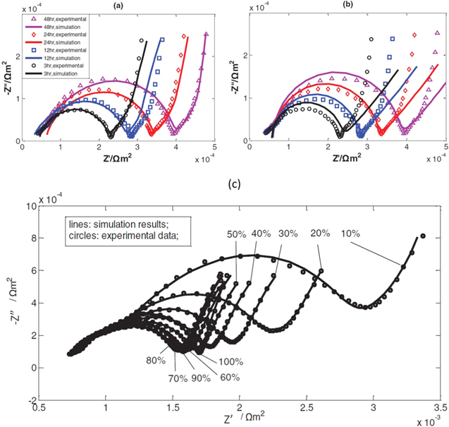
Figure 16. Fitting of the impedance response of a LiCoO2 particle with a diameter of  at different storage time with the electrode potential held at 4.0 V (vs
  /Li) using (a) the model treating the single particle as a spherical agglomerate, cf Eq. 178, and (b) the model neglecting electrolyte transport inside the single particle and using a Warburg impedance for diffusion.
65
(c) Fitting of the impedance response of a LiNi1/3Mn1/3Co1/3O2 porous cathode at different states of charge.
66
Reproduced with permission from The Electrochemical Society.
/Li) using (a) the model treating the single particle as a spherical agglomerate, cf Eq. 178, and (b) the model neglecting electrolyte transport inside the single particle and using a Warburg impedance for diffusion.
65
(c) Fitting of the impedance response of a LiNi1/3Mn1/3Co1/3O2 porous cathode at different states of charge.
66
Reproduced with permission from The Electrochemical Society.
Download figure:
Standard image High-resolution imageWhole electrode
In the section of extension in physics, we have obtained a general expression, Eq. 64, for the impedance response of porous electrodes considering mass transport in both electrode and electrolyte phases. This formula can be applied to model the impedance response of various kinds of battery electrodes, as detailed below. For three-scale battery electrodes made up of agglomerates, the agglomerate impedance, expressed in Eq. 181, is set as the local impedance element,  in Eq. 64. For two-scale battery electrodes made up of primary particles, Eqs. 178 and 180 are set as
  for the case with and without a SEI film covering primary particles, respectively. In Ref. 66, Huang et al. developed a three-scale impedance model for a LiNi1/3Mn1/3Co1/3O2 porous cathode. The model was parameterized with experimental data at a series of state of charge (SOC) measured using a reference electrode. As shown in Fig. 16c, the model agrees well with experiments over a wide range of SOC, and close examination of the resultant parameters lend further credence to the validity of the model.
Other models
Published in 2000, the MDDN (shorthand for Meyers-Doyle-Darling-Newman) model describes the impedance response of a porous electrode consisting of intercalation particles on two scales. 49 On the microscopic scale, the impedance of a single intercalation particle is phenomenologically described using an equivalent electric circuit of which some parameters are further derived from physical laws. On the macroscopic scale, the impedance of a porous electrode is described using the transmission line model taking into account both ionic conduction in the electrolyte phase and electronic conduction in the electrode phase. The MDDN model has following inadequacies. Firstly, the two-scale MDDN model cannot adequately describe porous electrodes that are composed of agglomerates and have a three-scale structure. Secondly, the physical meanings of the electric circuit and its elements describing the SEI film are elusive. Thirdly, ion transport in the electrolyte phase is described using the Ohm's law which considers migration only, while diffusion and the concentration gradient are neglected. The second limitation has been coped with by considering details of ion transport in the SEI film by Dees et al. 150,151 and Single et al. 152 The third limitation has been amended by Doyle et al. who numerically solved the full Newman model, 153 and by White et al. who provided analytical results. 67,152,154
The White group at University of South Carolina has been striving to develop analytical solutions for the impedance response of battery electrodes. In 2004, Devan and White obtained an analytical expression for the porous electrode with intercalation reactions. 154 The Devan-White model employs the concentrated solution theory for ion transport in the electrolyte phase and the Butler-Volmer equation for charge transfer reactions, but neglects diffusion in the solid phase. The synthetic impedance simulated using the model shows an arc in low frequency range corresponding to the electrolyte phase diffusion. Later on, Sikha and White complemented the Devan-White model by including solid-phase diffusion, presenting a comprehensive impedance model for two-scale battery electrodes. 67,152
The first limitation of the MDDN model was resolved by Huang et al.
65,66
They developed a three-scale impedance model for battery electrodes composed of agglomerates which are treated as spherical porous electrodes. A salient feature of the three-scale impedance model is that a 22.5° line exists in high frequency range, rather than a 45° in classical impedance models of porous electrodes. Of note, 22.5° and 11.25° lines in high frequency range have also been obtained by Itagaki et al. for the double- and triple-scale pore structures,
114
see a discussion in chapter 9.1.3 in Lasia's book.
15
In a more general sense, the impedance response of a n-scale porous electrode shows a  line in high frequency range. In other words, the number of scales of the porous electrode may well be calculated as
  with
with  being the angle of the inclined line in high frequency range. Generally,
  can be nonintergal. Besides the extension in the structure scale, the model developed by Huang et al. also features the coupling of double layer charging and charge transfer reactions and the detailed description of the SEI film.
65
In a more recent study, Huang and Zhang developed a general model for impedance response of various kinds of porous electrodes.
50
Applied to battery electrodes, the Huang-Zhang model is reduced to the earlier Sikha-White model. Furthermore, the Huang-Zhang model accounts for in-plane and through-plane pore size distribution, and obtains analytical solutions for several limiting cases, as discussed before. We note that in the field of time-domain modeling, Farrell et al. developed a three-scale model for primary alkaline battery cathode,
155
and later extended it to a LiFePO4 electrode.
156
can be nonintergal. Besides the extension in the structure scale, the model developed by Huang et al. also features the coupling of double layer charging and charge transfer reactions and the detailed description of the SEI film.
65
In a more recent study, Huang and Zhang developed a general model for impedance response of various kinds of porous electrodes.
50
Applied to battery electrodes, the Huang-Zhang model is reduced to the earlier Sikha-White model. Furthermore, the Huang-Zhang model accounts for in-plane and through-plane pore size distribution, and obtains analytical solutions for several limiting cases, as discussed before. We note that in the field of time-domain modeling, Farrell et al. developed a three-scale model for primary alkaline battery cathode,
155
and later extended it to a LiFePO4 electrode.
156
Other notable progress in theoretical modelling of impedance response of battery electrodes includes the treatment of phase transition by Ciucci and Lai, 157 and Gambhire et al., 158 the consideration of active particle morphology and electrode microstructure by Chen and Mukherjee, 159 the description of dendrite growth by Talian et al., 160 and the detailed discussion of the SOC-dependence by Gruet et al. 161 and Schönleber et al. 162 Specifically, Ciucci and Lai employed the Cahn–Hilliard framework to describe phase transition and the small signal perturbation approach to obtain impedance response, 157 while Gambhire et al. employed the core–shell model to describe phase transition. 158
Combined theory and experimental characterization
Although EIS is routinely applied in battery investigations, interpretation of the results using a physical impedance model is relatively rare. Herein, instead of presenting a comprehensive survey of relevant activities, which has been attempted in recent reviews, 22,163 we highlight several exemplary works filtrated through our eyes.
Lindbergh et al. employed EIS to investigate the aging mechanism of a LixNi0.8Co0.15Al0.05O2 porous electrode. 164,165 In so doing, they developed a physical impedance model based on the Newman model, featuring consideration of the realistic multilayer structure, size distribution of active particles in two shapes (spheres and flakes). EIS measurements were conducted using a three-electrode setup with flexible temperature and pressure control. EIS data were interpreted using their physical impedance model. They found that the impedance evolution along aging can be attributed to loss of active particles, increased local contact resistance between the active material and the conductive carbon, and increased resistance of a layer on the current collector. Recently, Zhou et al. 166 employed the physical impedance model developed by Huang et al. 66 to identify the mechanism of power fade of lithium-ion batteries, revealing that the electrolyte phase transport is the major cause.
EIS has also been proven powerful in assessing ion transport properties in battery porous electrodes. For this purpose, special design of the experimental setup is usually required. Roling et al. 167 and Latz et al. 168 determined the transference number of Li+ in electrolyte from very-low frequency impedance measured on a symmetric Li∣electrolyte∣Li cell. Gasteiger et al. determined the tortuosity of a battery porous electrode from the impedance measured under a blocking electrode configuration, which is realized by using a non-intercalating electrolyte. 169
Polymer electrolyte fuel cells
Polymer electrolyte fuel cells (PEFCs) have broad prospect in mobile and stationary power sources. Electrochemical impedance spectroscopy (EIS) is one of the most powerful in situ characterization tools for PEFCs, featuring non-destructive separation of kinetic and transport processes in a wide frequency range. It has been well recognized that unambiguous interpretation of EIS spectra requires models. Equivalent electrical circuit (EEC) model, dating back to Randles model 170,171 in 1940s (note that the Randles model is well grounded on physics but represented in electrical circuits) and enjoying wide usage owing to its simplicity, has limitations due to the polysemy and uncertainties in building models, and the missing link between EEC parameters and physical properties. Consequently, there has been a clear need for physical impedance models of PEFC. A list of symbols used in this section is given in Table VIII.
In this direction, a seminal work was conducted by Springer et al. in 1996, 172 who numerically calculated the impedance response of a PEFC model 42 developed earlier. The next decisive development was made by Eikerling and Kornyshev 48 in 1999. The Eikerling-Kornyshev model captures the essential processes in a PEFC in a much simpler formulation compared to the model developed by Springer et al., allowing analytical solutions to be obtained in several cases. Analytical expressions with rigorous physical origins greatly facilitate in-depth analysis of the impedance response of PEFCs. A wide variety of improvements over the original Eikerling-Kornyshev model strive to account for a plethora of complexities in PEFC. Among these, Kulikovsky has been making systematic contributions. 10–12,15–17,21,22,24–31,35–44
In what follows, we first present a general theory describing major physico-chemical processes in the porous electrode of PEFC, then transform these equations into dimensionless form, and then implement Fourier transform to set the stage for subsequent derivation of impedance response. Both analytical and numerical solutions are obtained for several limiting cases, and experimental relevance is discussed with reference to selected experimental studies. Other models beyond the above theoretical framework are reviewed separately. Our systematic exposition presented below closely follows theoretical works of Kulikovsky. 10–12,15–17,21,22,24–31,35–44 In addition to the systematic compilation, we have re-derived and implemented all models by ourselves with the MATLAB code provided in SI. Please refer to Table VIII for the list of symbols used in this section.
Physics and impedance model
Physics in PEFC porous electrodes
A PEFC consists of an anode where hydrogen is oxidized to protons,  a proton-conducting membrane responsible for proton conduction, electrical insulation and water transport, and a cathode where oxygen from the gas diffusion layer reacts with protons and electrons forming water, namely, via the oxygen reduction reaction (ORR),
  As the ORR constitutes the largest solo voltage losses in a PEFC, most attention has been paid to the cathode.
At the cathode, multi-dimension (thickness direction and along-channel direction), multi-media (CCL (cathode catalyst layer), GDL (gas diffusion layer) and gas flow channel), multi-component (oxygen, proton, electron and water) transport is coupled with the ORR. Schematic illustration of overpotential, proton, electron current density and gas concentration profiles at the cathode is depicted in Fig. 17. Water transport process is neglected and the effect of water is taken into account in the effective oxygen diffusion coefficient and the proton conductivity, assuming a uniform distribution of water saturation in pores and water content in ionomer.

Figure 17. Schematic illustration of the cathode side of PEFC with single air channel. ( is the through-plane coordinate from the membrane to the channel side and
  is the flow channel coordinate from the inlet to the outlet.
  is the thickness of catalyst layer,
  is the thickness of gas diffusion layer and
  is the length of air channel.
  is the dimensionless local proton current density,
  is the dimensionless local electron current density,
  is the dimensionless local oxygen concentration in the CCL,
  is the dimensionless local oxygen concentration in the GDL,
  is the dimensionless local oxygen concentration in the channel,
  is the dimensionless local ORR overpotential in the CCL.).
Download figure:
Standard image High-resolution imageThe full problem is simplified to a quasi-2D (1D + 1D) problem. The CCL is described along the through-plane direction, where the ionic, electronic, and faradaic current densities are correlated via the charge conservation law,
Here,  is a flux term from the ORR,
  is the volumetric double-layer capacitance (F cm−3),
  is time,
  is the local proton current density (A cm−2),
  is the distance from the membrane (m),
  is the volumetric exchange current density (A cm−3),
  is the local oxygen concentration in the CCL (mol m−3),
  is the reference oxygen concentration (mol m−3),
  is the Tafel slope (mV).
  is the local ORR overpotential given by
  where
where  is the potential in the ionic-conducting phase,
  is the potential in the electronic phase and
  is the equilibrium ORR potential. A transference number of 0.5 is used in the Butler-Volmer equation. The model is generic for other values of the transference number, but some of the analytical solutions rely on the specific value of 0.5.
Based on the Ohmic law,  is further given by,

with  being the CCL proton conductivity. Note that there is no proton flux in the GDL. As the ORR is the proton-coupled electron transfer reaction, the generation/consumption of protons should be equal to that of electrons, namely,

where  is electron current density described using the Ohmic's law with
  being the electron conductivity of CCL. The sum of local proton and electron current density is equal to the cell current density
  namely,
  As there is no proton flux in the GDL, Eq. 184 indicates readily that
  in the GDL. As for oxygen transport in the CCL and GDL, only the through-plane direction is considersed,

with  being the effective oxygen diffusion coefficient, and
  a flux term.
  equals
  in the CCL and
  in the GDL, and
  in the CCL and zero elsewhere.
The other dimension is the along-channel direction. Neglecting the rib/channel effect of flow field and assuming a plug gas flow with a constant velocity along the channel, the oxygen transport is described by,

Here  is the local oxygen concentration in the channel,
  is the distance from the channel inlet,
  is the flow velocity,
  is the channel depth,
  is the thickness of CCL and
  is the thickness of GDL.
Dimensionless equation set
The equation set consisting of Eqs. 182–186 is normalized to,

using dimensionless variables,
Here  is the channel length. Additional care should be paid to different length scales used for
  and
and  In addition,

are the reference values for time, current density and diffusion coefficient, respectively. A dimensionless reaction penetration depth is given by,

The characteristic time of oxygen concentration variation in the CCL and GDL is given by,

The oxygen stoichiometry reads,

where  is the inlet oxygen concentration. The characteristic time of oxygen concentration in the channel is given by,

and  is the ratio of electron to proton conductivity,

When analyzing the impedance response, we introduce the dimensionless impedance  and the dimensionless angular frequency
  as follows.

Here  is the impedance and
  is the angular frequency.
The boundary conditions for the system
61–66
are as follows. At the interface between the membrane and the CCL,  the ionic-phase potential is zero and set as the reference potential, namely,

and the electronic current is zero as electrons cannot go through the membrane, namely,

and the oxygen flux is zero since the oxygen cannot penetrate the membrane, namely,

At the CCL and the GDL interface,  the proton current is zero as protons cannot penetrate the GDL, namely,

and the electronic phase potential is fixed, which is usually the independent variable controlled in EIS measurement,

and the oxygen concentration distribution is continuous,

where  and
and  denote the left and right side of the CCL/GDL boundary, and the oxygen flux is equal on both sides of the interface,

At the GDL and air channel interface,  the oxygen concentration distribution is continuous,

At the air channel inlet,  the dimensionless oxygen concentration is fixed at 1,

Impedance model
Impedance response can be obtained by applying a small-amplitude harmonic perturbation to steady-state conditions. Let 


 and
and  be the steady-state solutions to Eqs. 187–192 and


 and
and  be the corresponding perturbations. Performing Fourier transform to the control equations given in Eqs. 187–192 subtracting the steady-state parts, and linearizing the nonlinear terms, we get a system of linear equations for the perturbed variables,

The boundary conditions for the equation system Eqs. 210–215 are as follows. At the interface between the membrane and the CCL,  where the reference potential is defined, the perturbation of ionic-phase potential is naturally zero,

and according to Eqs. 202–209, we have,


Thus, the cell impedance can be obtained using ohmic law,
The latter equality holds true as the current is contributed exclusively by electron conduction at  If we neglect electron conduction resistance when
  Eq. 211 is eliminated and Eq. 210 becomes

and the boundary conditions Eqs. 219 and 220 are now,

The cell impedance Eq. 225 now reads,
as the current is contributed exclusively by proton transport at 
Solutions and applications
PEFC enjoys a rich variety of operation conditions and cell configurations, e.g. the current density, gas stoichiometry, gas flow rate, properties of membrane electrode assembly (MEA), cell size and channel design etc. Under different circumstances, the theory expressed in Eqs. 187–192 can be simplified to different extent by neglecting one or several terms or even equations. In the following, we are to obtain analytical impedance expressions or numerically calculate the impedance for each limiting case and then to discuss its application to PEFC characterization and diagnosis. As shown in Table VI, six limiting cases are differentiated based on the transport phenomena described, and each case is further separately discussed under different reaction conditions.
Case 1: Proton conduction in the CCL
Table VI. Definition of six limiting cases in terms of mass transport processes.
| Case Number | Mass Transport in the CCL | ||||
|---|---|---|---|---|---|
 Conduction Conduction |
 Conduction Conduction | O2 Transport | O2 Transport in the GDL | O2 Transport in the Channel | |
| 1 | √ | x | x | x | x |
| 2 | √ | √ | x | x | x |
| 3 | √ | x | √ | x | x |
| 4 | x | x | x | √ | x |
| 5 | √ | x | √ | √ | x |
| 6 | √ | x | √ | √ | √ |
This limiting case focuses on proton conduction, in absence or presence of ORR, in the CCL only, while neglecting gas transport in the channel, GDL and CCL and electron conduction in the CCL. A PEFC operating at H2/N2 atmosphere neatly fits this case. In order to meet this limiting case under H2/O2 atmosphere, the cell should be made as uniform as possible in in-plane direction, fed with a sufficiently large gas stoichiometry  and operated at a current density
  that is much smaller than the diffusion-limited current densities for oxygen transport in the CCL
  and GDL
  namely,
  In addition, the electron conductivity
  should be much larger than the proton conductivity
  namely,
  or
or  to justify the neglect of electron conduction. In the following, we will discuss the impedance response in these circumstances, separately.
Blocking electrode
When the cathode is fed with nitrogen and the electrode potential is adjusted to be within the double-layer region, there is no charge transfer reaction at the electrode/electrolyte interface (EEI). We are then left with proton transport in the CCL which is described using the standard de Levie model. The impedance expression of this simple case is Ref. 50

where  is the volumetric area of the EEI, and
  is the local impedance at the EEI.
In the limit of  Eq. 229 is asymptotic to

which is represented by a 45° line in the Nyquist plot. In the limit of  Eq. 229 is asymptotic to

which is represented by a vertical line in the Nyquist plot. The full Nyquist plot of impedance response given by Eq. 229 is shown as the black line in Fig. 19. The proton conductivity is related with the real part of  via
via

By fitting the experimental impedance spectrum with Eq. 229, we can obtain 
 and
and  Pickup et al.
173
used this method to compare the proton conductivity of electrodes with and without ionomer in the CCL. Results show that the ionomer-containing CCL possesses a higher proton conductivity, bringing larger active area and thus better performance. Gasteiger et al.
174,175
employed this method to measure
Pickup et al.
173
used this method to compare the proton conductivity of electrodes with and without ionomer in the CCL. Results show that the ionomer-containing CCL possesses a higher proton conductivity, bringing larger active area and thus better performance. Gasteiger et al.
174,175
employed this method to measure  of the CCL with various ionomer/carbon weight ratios (I/C ratios) at different relative humidities (RHs). Using the same method, Zhang et al.
176
investigated the evolution of
of the CCL with various ionomer/carbon weight ratios (I/C ratios) at different relative humidities (RHs). Using the same method, Zhang et al.
176
investigated the evolution of  of PEFC during cold start.
Small current density
The assumption of fast oxygen transport in the channel, GDL and CCL leads to  and
and  simplifying Eq. 226 to

Furthermore, when the current density is much smaller than the characteristic current density for proton conduction,  the steady-state distribution of the overpotential, controlled by Tafel kinetics, is given by
177
the steady-state distribution of the overpotential, controlled by Tafel kinetics, is given by
177
where  is the solution of
  Provided
  in Eq. 234, Eq. 233 becomes
When the current density is sufficiently small,  which is realized when the voltage is close to OCV, the second term in the bracket approaches
  Then, Eq. 235 closed with the boundary conditions given in Eq. 227 is analytically solved. resulting in the impedance expression of the real and imaginary parts given by
178
Then, Eq. 235 closed with the boundary conditions given in Eq. 227 is analytically solved. resulting in the impedance expression of the real and imaginary parts given by
178
where two coefficients are given by
In the limit of  Eqs. 236 and 237 are asymptotic to
  Thus, the high-frequency impedance is manifested as a 45° straight line in the Nyquist plot, associated with the proton conduction in the CCL. In the limit of
  Eqs. 236 and 237 are asymptotic to
  and
and  It implies that the impedance plot converges to a pure resistance on the real axis in the low-frequency limit. The low-frequency impedance is manifested as an arc related with the ORR in the CCL. The full Nyquist plot of impedance response is shown in Fig. 18a, and it well fits the numerical results. Two values of
  are compared. When
  grows from 1 to 866, meaning much faster proton conductivity, the 45° line diminishes while the arc size remains constant.
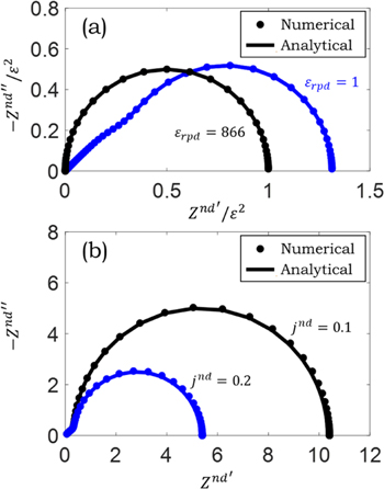
Figure 18. Nyquist plot of impedance response of the CCL for the limiting case 1 with ORR. (a) The PEFC is kept at OCV. The curve for  clearly shows a 45° line in high-frequency region, which disappears for
  Note that the axis is
  (b) The PEFC operates at a small current density. The 45° line in high-frequency region overlaps for different current densities, while the arc related with the ORR decreases with increasing the current density.
  is the real part of the dimensionless impedance, and Znd'' is the imaginary part of the dimensionless impedance, and
  is the dimensionless current density.
Download figure:
Standard image High-resolution imageFitting the experimental EIS at OCV with Eqs. 236 and 237, one can obtain  and
and  of ORR, and, principally speaking,
  in the CCL as well. However, the ORR usually obscures the 45° line corresponding to proton transport in the CCL, except under ultra-dry operation condition or for electrodes with poor proton conduction,
179
making it difficult to extract the proton conductivity with high confidence. Consequently, Eqs. 236 and 237 are usually used to determine ORR parameters, such as charge-transfer resistance
180
and the activation energy of ORR.
181
in the CCL as well. However, the ORR usually obscures the 45° line corresponding to proton transport in the CCL, except under ultra-dry operation condition or for electrodes with poor proton conduction,
179
making it difficult to extract the proton conductivity with high confidence. Consequently, Eqs. 236 and 237 are usually used to determine ORR parameters, such as charge-transfer resistance
180
and the activation energy of ORR.
181
When the current density falls into the range of  ≪
≪  ≪
≪  we then neglect the unity under the square root of the second term in the bracket of Eq. 235 and replace the cos2 term with 1, thus
  Then, the impedance expression becomes
182–184
Then, the impedance expression becomes
182–184
where two coefficients are
In the limit of  Eqs. 239 and 240 are asymptotic to
  as the same with Eqs. 236 and 237. In the limit of
  Eqs. 239 and 240 are asymptotic to
  and
and  implying that the impedance plot converges to a pure resistance associated with the charge transfer on the real axis in the low-frequency limit, and the charge transfer resistance monotonically decreases with increasing the cell current density. The full Nyquist plot of impedance response given by Eqs. 239 and 240 is shown in Fig. 18b, consisting of a 45° line in high-frequency range and an arc associated with the ORR in low-frequency range. When the cell current density increases, the low-frequency arc shrinks while the 45° straight line remains constant. The model developed here may well be used to interpret the impedance spectrum measured at small current density, for example, the data reported by Baker et al.,
185
Stamper et al.
186
and Lindbergh et al.
187
implying that the impedance plot converges to a pure resistance associated with the charge transfer on the real axis in the low-frequency limit, and the charge transfer resistance monotonically decreases with increasing the cell current density. The full Nyquist plot of impedance response given by Eqs. 239 and 240 is shown in Fig. 18b, consisting of a 45° line in high-frequency range and an arc associated with the ORR in low-frequency range. When the cell current density increases, the low-frequency arc shrinks while the 45° straight line remains constant. The model developed here may well be used to interpret the impedance spectrum measured at small current density, for example, the data reported by Baker et al.,
185
Stamper et al.
186
and Lindbergh et al.
187
The proton conduction of CCL exhibits a 45° straight line in impedance spectrum, as discussed above. However, the straight line could deviates from 45° slope when considering  distribution through CCL depth, caused by non-uniform ionomer distribution. Reshetenko and Kulikovsky
188
introduced a distributed electrolyte proton conductivity
distribution through CCL depth, caused by non-uniform ionomer distribution. Reshetenko and Kulikovsky
188
introduced a distributed electrolyte proton conductivity  with
with  into Eq. 183. Thus, in high-frequency region, Eq. 233 transfers to

Solving Eq. 242 with the boundary conditions given in Eq. 227, they write the impedance expression in high-frequency region as
where

and 
 are the Bessel functions of the first and second kind, respectively. Then, they fitted Eq. 243 to the HF part of the experimental Nyquist spectra at the open–circuit conditions,
189
and obtained the characteristic scale of
are the Bessel functions of the first and second kind, respectively. Then, they fitted Eq. 243 to the HF part of the experimental Nyquist spectra at the open–circuit conditions,
189
and obtained the characteristic scale of  decay along
Case 2: Electron and proton conduction in the CCL.
This limiting case focuses on proton and electron conduction, without or coupled with ORR, in the CCL only, while neglecting gas transport in the channel, GDL and CCL. Compared to the case 1, another transport process, namely electron conduction, comes into play in the case 2. Most often, the electron conductivity is usually one to two orders of magnitude larger than the proton conductivity in the CCL.
190
However, in some occasions, e.g. Pt-free electrodes or degraded CCL due to carbon corrosion, the electron conductivity decreases greatly and electron conduction exerts a noticeable effect on the impedance spectrum, this limiting case deals with such occasions. The operation conditions for this case are nearly the same as those fulfilling the limiting case 1: a PEFC operating at H2/N2 atmosphere or H2/O2 atmosphere with a small current density,  .
.
Blocking electrode
When the cathode is fed with nitrogen and the electrode potential is adjusted to be within the double-layer region, there is no charge transfer reaction at the EEI. We are then left with proton and electron transport in the CCL which can be described using transmission line (TML) model. This case corresponds to the case two in the section of "extension in physics," and the impedance expression reads 50
with

where  is the local impedance at the EEI.
In the limit of  Eq. 245 is asymptotic to
which is represented by a 45° line in the Nyquist plot. When  Eq. 247 simplifies to Eq. 230. In the limit of
  Eq. 245 is asymptotic to

which is represented by a vertical line in the Nyquist plot. When  Eq. 248 simplifies to Eq. 231. The length of the real part of the 45° straight line
  is obtained by subtracting Eq. 247 from Eq. 248,
which reaches the minimal value when the ratio of electron to proton conductivity  The full Nyquist plot of impedance response given by Eq. 245 is shown in Fig. 19.
  dictates
  via Eq. 249, and
 can be extracted from high-frequency resistance via


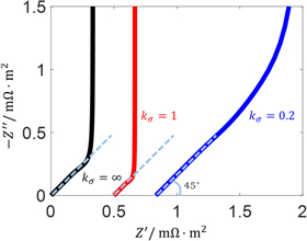
Figure 19. The Nyquist plot of the CCL under H2/N2 atmosphere for limiting cases 1 and 2. For comparison, the ratio of electron to proton conductivity  is set to 0.2, 1 and infinite (limiting case 1), respectively. Parameters used in the simulation are taken from Ref. 50.
Download figure:
Standard image High-resolution imageIn Fig. 19, three impedance spectra are compared to show the effect of  When
When  reduces from infinite via 1 to 0.2, the spectrum shifts right towards and
  decreases first, and then increases much, which is consistent with the analysis above. Very recently, this model has been used to extract the electron and proton conductivity of a Fe–N–C electrode by Reshetenko et al.
191
decreases first, and then increases much, which is consistent with the analysis above. Very recently, this model has been used to extract the electron and proton conductivity of a Fe–N–C electrode by Reshetenko et al.
191
Small current density
In the small current density regime, fast oxygen transport is assumed in the channel, GDL and CCL, namely,  and
and  We can transform Eqs. 210–211 to
Furthermore, when the current density  is much smaller than the characteristic current density for proton (
 ) and electron (
 ) conduction in the CCL,
  we can neglect the static overpotential distribution through the CCL depth, namely,
  Thus, Eqs. 252–253 closed with the boundary conditions Eqs. 219–220 can be analytically solved, resulting in the impedance expression given by
192
Thus, Eqs. 252–253 closed with the boundary conditions Eqs. 219–220 can be analytically solved, resulting in the impedance expression given by
192
where
When the current density is sufficiently small,  which is realized when the voltage is close to the OCV, we substitute
  into Eqs. 255–256 and obtain


In the limit of  Eq. 254 is asymptotic to

Rearranging this equation as

indicates that the CCL has a purely ohmic resistance, which is equivalent to ionic and electronic resistances in parallel connection. In the limit of  Eq. 254 is asymptotic to

Here, the first term is the faradaic resistance, and the second and third term are the proton and electron conduction resistivities, respectively. The full Nyquist plot of impedance response given by Eq. 254 is shown in Fig. 20a, and it well fits the numerical solution.

Figure 20. The Nyquist plot of the CCL in limiting case 2. For comparison, the ratio of electron to proton conductivity  is set to 0.2, 1 and infinite, respectively. (a) At OCV. The dimensionless reaction penetration depth
  is set to 1 to emphasize the proton and electron conduction. (b) At small current density. The current density
  is set to 0.1. (c) The high-frequency part of the spectra in (b).
  is the real part of the dimensionless impedance, and
  is the imaginary part of the dimensionless impedance.
Download figure:
Standard image High-resolution imageWhen the current density falls into the range of  ≪
≪  we employ the Tafel equation to describe the relation between overpotential and current density,
177
we employ the Tafel equation to describe the relation between overpotential and current density,
177

Substituting Eq. 262 into Eqs. 255 and 256 gives 192


In the limit of  we get the same simplification as in the OCV circumstance. In the limit of
  Eq. 254 is asymptotic to

Compared to Eq. 261, the faradaic resistance is determined by  instead of
  The full Nyquist plot of impedance response given by Eq. 254 is shown in Figs. 20b and 20c. The model of this case may well be used to interpret the impedance spectrum measured on Fe–N–C cathodes with different catalyst loadings and I/C ratios by Malko et al.
193
and Reshetenko et al.
194
The full Nyquist plot of impedance response given by Eq. 254 is shown in Figs. 20b and 20c. The model of this case may well be used to interpret the impedance spectrum measured on Fe–N–C cathodes with different catalyst loadings and I/C ratios by Malko et al.
193
and Reshetenko et al.
194
Case 3: Proton and oxygen transport in the CCL
This limiting case focuses on proton conduction and oxygen transport, coupled with ORR, in the CCL only, while neglecting gas transport in the channel and GDL, and electron conduction in the CCL. To meet this limiting case, the cell should be made as uniform as possible in the in-plane direction, fed with a sufficiently large gas stoichiometry  and operated at a current density
  that is much smaller than the diffusion-limited current densities for oxygen transport in the GDL
  namely,
  In addition, the electron conductivity
  should be much larger than the proton conductivity
  namely,
  or
or  to justify the neglect of electron conduction. To get the analytical expressions, it is additionally assumed that the cell current density is much smaller than the characteristic current densities for proton,
  Thus, the overpotential is taken constant through the CCL depth,
Fast oxygen transport in the CCL
When the oxygen transport in the CCL is so fast that the characteristic current density of oxygen transport  is much larger than the working current density
  namely,
  Tafel equation is used to describe the relation between static overpotential and current density, as shown in Eq. 262. Then, Eqs. 226 and 212 are asymptotic to

Equations 266–267 closed with the boundary conditions Eqs. 227 and 221 are analytically solved. 195 The full solution is shown in Eqs. (S74)–(S78) in the SI.
In the limit of  we retrieve
  as in the case 1. In the limit of
  the impedance expression is asymptotic to

Compared to Eq. 265, the new third term corresponds to oxygen transport resistance in the CCL. The full Nyquist plot of impedance response described by Eq. (S74) is shown in Fig. 21a. Four groups of impedance spectrum are compared to examine the effect of  We find that the impedance arc expands with decreasing
  and the analytical solution fits numerical solutions well for high
  Equation 268 implies that
  is able to be determined from impedance experiments with high confidence. In so doing, the effect of gas transport in the GDL should be minimized, for example, by using gold mesh to replace GDL. Till now, few experimental work corresponding to this case has been done.
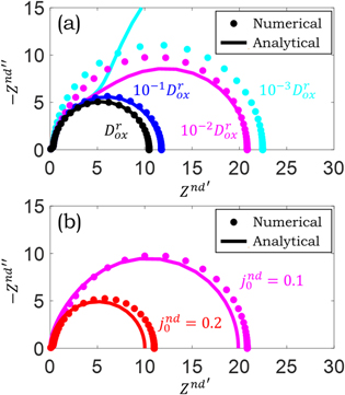
Figure 21. The Nyquist plot of the CCL impedance in the limiting case 3. (a) The current density  and the effective oxygen diffusion coefficient in the CCL is varied with the reference value of
  cm2 s−1. (b)
  is set to
  and two current densities
  are compared.
  is the real part of the dimensionless impedance, and
  is the imaginary part of the dimensionless impedance.
Download figure:
Standard image High-resolution imageSluggish oxygen transport in the CCL
When the oxygen transport is sluggish and the corresponding characteristic current density  is smaller than the working current density
  namely,
  the steady-state overpotential and oxygen concentration are written as Ref. 196
Here an empirical double Tafel slope is used. Substituting Eq. 269 into Eqs. 226 and 212 and using the boundary conditions Eqs. 227 and 221, we calculate the impedance as Refs. 196, 197
where  is the Warburg-like impedance of the transport layer of a finite length thickness and
  is its static limit,
In the limit of  Eq. 270 approaches to
  In the limit of
  Eq. 270 approaches to

The factor  describes the doubled Tafel slope due to poor oxygen transport in the CCL.
198
The full Nyquist plot of impedance response given by Eq. 270 is shown in Fig. 21b. In high-frequency region, the 45° straight line maintains in the numerical spectrum, while disappears in the analytical spectrum due to the assumption of neglecting the proton conduction. Two groups of impedance spectrum are compared to examine the effect of
describes the doubled Tafel slope due to poor oxygen transport in the CCL.
198
The full Nyquist plot of impedance response given by Eq. 270 is shown in Fig. 21b. In high-frequency region, the 45° straight line maintains in the numerical spectrum, while disappears in the analytical spectrum due to the assumption of neglecting the proton conduction. Two groups of impedance spectrum are compared to examine the effect of  We find that when
  is doubled, the arc size is halved. Equation 270 provides a way to measure
  in the CCL from impedance experiments, especially for PGM-free electrodes who is one order of magnitude thicker than traditional ones. Malko et al.
193
and Reshetenko et al.
194
have measured the impedance of M–N–C (M=Fe, Co, Ni, Mn etc.) cathodes at moderate current densities. Fitting these results with the analytical model shown in Eq. 270, one is able to obtain
in the CCL from impedance experiments, especially for PGM-free electrodes who is one order of magnitude thicker than traditional ones. Malko et al.
193
and Reshetenko et al.
194
have measured the impedance of M–N–C (M=Fe, Co, Ni, Mn etc.) cathodes at moderate current densities. Fitting these results with the analytical model shown in Eq. 270, one is able to obtain 
 and
and  in the CCL.
Case 4: Oxygen transport in the GDL
This limiting case concentrates on the oxygen transport in the GDL, coupled with the ORR in the CCL, while neglecting gas transport, proton and electron conduction in the CCL. To satisfy this limiting case, the cell should be made as uniform as possible in the in-plane direction, fed with a sufficiently large gas stoichiometry  and operated at a current density
  that is much smaller than the characteristic current densities for proton (
 ) and electron conduction (
 ) and for oxygen transport (
 ) in the CCL,
  Furthermore, to stress the effect of oxygen transport in the GDL, the diffusion-limited current density for oxygen transport in the CCL should be much larger than that of GDL, namely,
  Thus, the distributions of current density, oxygen concentration, overpotential through the CCL are safely neglected, that is, CCL is simplified to a thin film electrode with a large roughness factor. Under these assumptions, Eq. 212 is omitted, and
  and
and  in Eq. 226 is replaced with
  and
and  respectively. Using the Tafel equation in Eq. 262, Eq. 226 reduces to

Integrating both sides of Eq. 226 through CCL depth with Eq. 183, we have

According to the mass conservation equation, the oxygen flux in the GDL equals the consumption rate in the CCL, then we have

Equations 274 and 213 closed with the boundary conditions Eqs. 275, 223 and 227 are analytically solved (shown in the SI), and then the expression for GDL impedance can be obtained, 199–201
The full Nyquist plot of impedance response given by Eq. 276 is shown in Fig. 22a. The analytical solution given in Eq. 276, based on the assumption of fast oxygen transport, fits the numerical solution well at higher  in the GDL. Equation 276 differs from the standard Warburg impedance describing diffusion in a layer of a finite thickness
  202
202


Figure 22. The Nyquist plot of the cathode electrode impedance for the limiting case 4. The effective oxygen diffusion coefficient in the CCL  is fixed at
  cm2 s−1. (a) The current density
  and the effective oxygen diffusion coefficient in the GDL is varied with the reference value of
  cm2 s−1. (b) The comparison between Eq. 276 and Warburg impedance.
  is fixed at
  and three current densities
  are compared.
  is the real part of the dimensionless impedance, and
  is the imaginary part of the dimensionless impedance.
Download figure:
Standard image High-resolution imageThe fundamental difference between Eqs. 276 and 277 exists in the factor  in the dominator of Eq. 276. The reason for this "non–Warburg" factor in Eq. 276 is explained as follows. Warburg impedance is derived based on the planar electrode assumption.
99
Since
in the dominator of Eq. 276. The reason for this "non–Warburg" factor in Eq. 276 is explained as follows. Warburg impedance is derived based on the planar electrode assumption.
99
Since  of planar electrodes is negligibly small, the transient term
  in Eq. 187 can be neglected, leading to the neglect of the last term in Eq.274, which corresponds the "non–Warburg" factor in Eq. 276. However, the electrochemical active surface of a porous electrode is two to three orders of magnitude higher than that of a planar electrode, therefore, the "non-Warburg" factor cannot be ignored for porous electrode. Approaching the static limit (
 ), Eq. 276 reduces back to the Warburg impedance when the cell is operated at low
  The comparison of the impedance spectra of Eqs. 276 and 277 is shown in Fig. 22a. Note that in the high-frequency region, the real part of
  is negative due to dominant "non–Warburg" factor. However, the total impedance consisting of
  and faradaic impedance is always positive. With increasing
  the difference in low-frequency region grows due to the factor,
  in the dominator of Eq. 276. In the limit of
  Eq. 276 approaches to

Then,  is related with
  via,
via,

To eliminate other factors coupled with oxygen transport in the GDL when determining  a possible strategy is to vary the GDL thickness, for example, by change the number of GDL layers.
203
Steinberger et al.
204
have measured the EIS of a PEFC at low-to-moderate current densities at a series of GDL thickness. Using the difference in
a possible strategy is to vary the GDL thickness, for example, by change the number of GDL layers.
203
Steinberger et al.
204
have measured the EIS of a PEFC at low-to-moderate current densities at a series of GDL thickness. Using the difference in  between different GDL thicknesses, one obtains
  via,
via,

Case 5: Proton and oxygen transport in the CCL and oxygen transport in the GDL
This limiting case considers the through-plane physical processes in the cathode. To satisfy this case, the cell should be made as uniform as possible in the in-plane direction, and fed with a sufficiently large gas stoichiometry  In addition, the electron conductivity
  should be much larger than the proton conductivity
  namely,
  or
or  to justify the neglect of electron conduction. To obtain analytical solutions, we assume the cell current is small enough,
  to insure that the oxygen concentration is
  and the overpotential fulfills Eq. 262. The controlling equations given in Eqs. 273, 212 and 213 closed with the boundary conditions Eqs. 275, 221–224 and 227 can be analytically solved, resulting in the impedance expression,
184,205,206
and the overpotential fulfills Eq. 262. The controlling equations given in Eqs. 273, 212 and 213 closed with the boundary conditions Eqs. 275, 221–224 and 227 can be analytically solved, resulting in the impedance expression,
184,205,206
where the coefficients and arguments are listed in Eqs. (S82)-(S103) in the SI. In the limit of  Eq. 281 approaches to

Compared to Eq. 268, the additional fourth term corresponds to the oxygen transport resistance in the GDL. The full Nyquist plot of impedance response given by Eq. 281 is shown in Fig. 23. Decreasing  we observe another impedance arc in low-frequency region, indicating larger oxygen transport resistance. Numerical calculation is needed to solve the model at arbitrary
  207,208
Equipped with this model, one is able to extract
207,208
Equipped with this model, one is able to extract 
 and
and  from experimental EIS. However, no experimental EIS result has been interpreted using this model yet.
Case 6: Proton conduction in the CCL and oxygen transport in the CCL, GDL and channel.
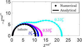
Figure 23. The Nyquist plot of the cathode electrode impedance for the limiting case 5. The current density  and the effective oxygen diffusion coefficient in the GDL is varied with the reference value of
  cm2 s−1. The effective oxygen diffusion coefficient in the CCL
  is fixed at
  cm2 s−1.
  is the real part of the dimensionless impedance, and
  is the imaginary part of the dimensionless impedance.
Download figure:
Standard image High-resolution imageThis limiting case treats both the through-plane processes, including proton and electron conduction and oxygen transport in the CCL and GDL, and the in-plane process, namely, oxygen transport along the channel. Compared to limiting case 5, this case adds the effects of oxygen flow in the channel. The intricate coupling between these processes makes Eqs. 189–192 intractable analytically, and numerical solutions are needed.
199,209–211
However, if ignoring diffusion process in the through-plane direction, Kulikovsky has obtained analytical expressions for oxygen transport in the channel.
212
In this case,  and
and  are constant at the same
  position,

 and
and  Integrating Eq. 226, we get

Substituting Eq. 275 into Eq. 214, we obtain

A good approximation for the oxygen concentration distribution along the channel at low-current at steady state is 213

Substituting Eqs. 283 and 285 into Eq. 284, and solving Eq. 284, we get the oxygen perturbation along the channel, as shown in Eq. (S94). Thus, the local impedance  of the cell can be obtained by substituting Eq. (S94) into Eq. 283 and dividing both sides by

where  is shown in Eq. (S95). At low current density,
  depends on the coordinate
  as Ref. 213
Substituting Eqs. 262 and 285 into Eq. 287, we obtain the global polarization curve of the cell,

Integrating Eq. 286 along the channel coordinate  we arrive at,

where  is shown in Eq. (S96) In the limit of
  Eq. 289 reduces to the faradaic impedance of the CCL,

In the limit of  we get the static resistance of the cell,

The full Nyquist plots of impedance response given by Eqs. 286 and 289, and numerical model are shown in Fig. 24. We find that the local impedance along the channel convolutes before emerging another channel-related impedance arc in low-frequency region, due to the spatial oscillation of the oxygen concentration, which has been observed in experiments by Schneider et al.
214,215
Reshetenko and Kulikovsky measured the local impedance spectrum of a segmented cell and fitted the model cell impedance to the experimental spectrum yields the parameters of individual segments, i.e., the shape of the cell physical parameters along the cathode channel.
209–211
By conducting impedance experiments and model fitting with different  and channel configuration, the effects of transport in channel and GDL could be distinguished, which is of great significance for the correct interpretation of impedance spectrum.

Figure 24. The Nyquist plot of the cathode impedance for the limiting case 6. The current density of the cell at the inlet region  and the effective oxygen diffusion coefficients in the CCL
  and GDL
  are fixed at
  cm2 s−1 and
  cm2 s−1, respectively. The oxygen stoichiometry
  is set to 2. The number near the curve represents the value of
  (a) The numerical local impedance spectra along the channel. (b) The analytical local impedance spectra along the channel corresponding to the local impedance expression Eq. 286. (c) The average impedance spectrum of the whole cathode.
  is the real part of the dimensionless impedance, and
  is the imaginary part of the dimensionless impedance.
Download figure:
Standard image High-resolution imageA summary and other models
In this section, we summarize the PEFC impedance theory presented above and complement it by reviewing other models developed in the literature. The six limiting cases share following assumptions: (1) water production and transport are not considered; (2) homogeneous structural, reaction and transport properties; (3) empirical description of the ORR using a single Butler-Volmer equation. The typical impedance spectra of limiting cases 1–6 are collected in Fig. 25, and the criteria of choosing these cases is listed in Table VII. In Fig. 25, we decompose the impedance spectrum of each case into several contributions. For instance, the total impedance  is separated into four contributions, namely, oxygen transport impedance in the channel
  oxygen transport impedance in the GDL
  oxygen transport impedance in the CCL
  and charge transfer impedance coupled with proton conduction
  It should be noted that there is always the problem of overfitting in extracting model parameters from experimental data. Consequently, it is important to report confidence interval of the fitted parameters, and to fit a set of experimental data instead of a single curve, if possible.

Figure 25. Typical impedance spectra for limiting cases 1–6.  is the total cathode impedance,
  is the oxygen transport impedance in the GDL,
  is the oxygen transport impedance in the CCL, and
  is the charge transfer impedance coupled with proton conduction, and
  is the charge transfer impedance coupled with proton and electron conduction.
Download figure:
Standard image High-resolution image
Table VII. The criterion of limiting cases 1–6.

|
Other models in the literature are categorized into three subjects: those related to modelling of the inductive loop in low frequency range, those involving the agglomerate scale, and those treating the impedance response of ultra-thin ionomer-free catalyst layers.
Table VIII. List of symbols in section 'Polymer electrolyte fuel cells'.
| Symbol | Description |
|---|---|

| Volumetric area of the EEI, 
|

| Tafel slope, mV dec−1 |

| Local oxygen concentration in the CCL, mol m−3 |

| Dimensionless local oxygen concentration in the CCL |

| Local oxygen concentration in the channel, mol m−3 |

| Dimensionless local oxygen concentration in the channel |

| Inlet oxygen concentration, mol m−3 |

| Reference oxygen concentration, mol m−3 |

| Volumetric double-layer capacitance, F cm−3 |

| Effective oxygen diffusion coefficient, m2 s−1 |

| Dimensionless effective oxygen diffusion coefficient |

| Reference value for diffusion coefficient, m2 s−1 |

| Oxygen diffusion coefficient in the GDL, m2 s−1 |

| Oxygen diffusion coefficient in CCL, m2 s−1 |

| Dimensionless oxygen diffusion coefficient in CCL, m2 s−1 |

| Equilibrium ORR potential, V |

| Dimensionless equilibrium ORR potential |

| Local current density, A cm−2 |

| Dimensionless local current density |

| Cell current density, A cm−2 |

| Electron current density, A cm−2 |

| Local proton current density, A cm−2 |

| Reference current density, A cm−2 |

| Bessel function of the first kind |

| Channel depth, m |

| Volumetric Exchange current density, A cm−3 |

| Thickness of GDL, m |

| Dimensionless thickness of GDL |

| Thickness of CCL, m |

| Channel length, m |

| Warburg-like impedance of the transport layer |

| Flux terms, 
|

| Time, s |

| Dimensionless time |

| Characteristic time of oxygen concentration variation in the CCL and GDL, s |

| Characteristic time of oxygen concentration in the channel, s |

| Reference value for time, s |

| Flow velocity, m s−1 |

| Distance from the membrane, m |

| Dimensionless distance from the membrane. |

| Bessel function of the second kind |

| Distance from the channel inlet, m |

| Dimensionless distance from the channel inlet |

| Impedance, 
|

| Oxygen transport impedance in the channel, 
|

| Oxygen transport impedance in the CCL |

| Oxygen transport impedance in the GDL, 
|

| Local impedance at the EEI, 
|

| Charge transfer impedance coupled with proton conduction, 
|

| Charge transfer impedance coupled with proton and electron conduction, 
|

| Warburg-like impedance of the transport layer of a finite length thickness, 
|

| Static resistance of the cell, 
|

| The dimensionless impedance. |

| The real part of the dimensionless impedance. |

| The imaginary part of the dimensionless impedance. |

| Coefficient in Eq. 238 |

| Coefficient in Eq. 238 |

| Local ORR overpotential, 
|

| Dimensionless local ORR overpotential |

| Potential in the ionic-conducting phase, V |

| Dimensionless the potential in the ionic-conducting phase. |

| Potential in the ionic-conducting phase, V |

| Potential in the electronic phase, V |

| Dimensionless potential in the electronic phase |

| Electron conductivity of CCL, 
|

| CCL proton conductivity, 
|

| Dimensionless reaction penetration depth |

| Oxygen stoichiometry |

| Ratio of electron to proton conductivity |

| Angular frequency, s−1 |

| Dimensionless angular frequency |
Inductive loop modeling
The impedance spectra measured in some circumstances exhibit a low-frequency inductive loop, 216,217 which cannot be explained using the models developed above. Three types of models were developed for interpreting the low-frequency inductive loop, the first type involves multiple step reactions with adsorbed intermediates on Pt surface, the second type involves platinum oxide growth, and the third type involves water transport.
In the first type, Bultel et al.
217
considered a three-step ORR mechanism, namely, 

 They attributed the inductive loop to the relaxation of intermediate adsorbed species, whereas such behavior is generally masked by oxygen diffusion in the case of the RDE. Neglecting the proton and oxygen transport losses, Kulikovsky
218
derived the analytical impedance model of the CCL considering the three-step ORR based on the Damjanovic dynamics of surface coverages.
They attributed the inductive loop to the relaxation of intermediate adsorbed species, whereas such behavior is generally masked by oxygen diffusion in the case of the RDE. Neglecting the proton and oxygen transport losses, Kulikovsky
218
derived the analytical impedance model of the CCL considering the three-step ORR based on the Damjanovic dynamics of surface coverages.
In the second type, Setzler et al.
219
considered a two-step mechanism for platinum oxide growth at terrace sites: 
 and one-step mechanism at edge sites:
  And they attributed the low-frequency inductive loop to the oxide poisoning. Cruz-manzo et al.
220,221
combined a two-step ORR mechanism,
And they attributed the low-frequency inductive loop to the oxide poisoning. Cruz-manzo et al.
220,221
combined a two-step ORR mechanism, 
 and a two-step platinum oxide growth mechanism,
 They studied the effect of hydrogen peroxide and platinum oxide formation on the low-frequency inductive loop.
In the third type, water production and removal are interlinked with the low-frequency inductive loop. Pivac et al. 216 proved this link by examining the cell impedance at various operating conditions, namely, different current densities, cell temperatures, gas humidities, air flow stoichiometries and backpressures. Wiezell et al. 222 modelled the low-frequency inductive loop using a single-phase model including the water transport in the membrane and the water-dependent proton conductivity in the electrodes. It is found that the membrane thickness and relative humidity shift the characteristic frequency and change the size of the inductive loop. Futter et al. 223 developed a 2D continuum physical model, incorporating non-isothermal, compositional multi-phase flow in both electrodes coupled with the transport of water, protons and dissolved gaseous species in the membrane. Besides, platinum oxides behave as site blockers, reducing the active area in their model. Modeling results show that the low-frequency induction is caused by humidity dependent ionomer properties and platinum oxide formation on the catalyst surface.
It is still unclear which of the three mechanisms is the main cause for the low-frequency inductive loop. Since platinum oxide formation occurs at high voltages and water transport effect becomes important at high current density and high RH, systematic impedance measurement at different voltages and RHs should be conducted to differentiate these mechanisms.
Agglomerate model
Agglomerate structure has been long before introduced as a representative element in macro-homogeneous model to account for the heterogeneous and microscopic details of the CL. The physical processes occurring at the agglomerate scale have been introduced in section 4.2.2, and a comprehensive review of agglomerate model in time-domain simulation has been provided by Huang et al.
135
For impedance modeling, as described in section 4.2.2, the oxygen concentration at the reaction interface is determined together by Fickian diffusion through the CCL, the dissolution of oxygen at the ionomer thin film surface, and the Fickian diffusion inside the agglomerate. Franco et al.
224
simplified the agglomerate structure to an ionomer-film-covered Pt/C surface and investigated the impedance response. Gerteisen et al.
225
introduced dissolution and diffusion equation of spherical agglomerate to determine the flux term  in Eq. 185. The CCL impedance arc at small current density doubled due to the extra gas transport in agglomerate. By using this model, the Henry and diffusion coefficient can be extracted with EIS experiments. However, unlike the secondary particles in LIBs, agglomerates are an ill-defined concept in PEFCs. In some cases, especially for ultra-thin catalyst layer, the agglomerate concept may lose its validity.
135
in Eq. 185. The CCL impedance arc at small current density doubled due to the extra gas transport in agglomerate. By using this model, the Henry and diffusion coefficient can be extracted with EIS experiments. However, unlike the secondary particles in LIBs, agglomerates are an ill-defined concept in PEFCs. In some cases, especially for ultra-thin catalyst layer, the agglomerate concept may lose its validity.
135
Impedance model of ionomer-free ultrathin catalyst layers (UTCLs)
UTCLs enable dramatic improvements in Pt utilization and activity over conventional CLs at ultra-low Pt loadlings. The ionomer-free structure requires proton conduction through water, mediated by electrostatic interactions of metal surface charge. 226 The electroneutrality assumption in electrolyte phase is no longer applicable and Poisson-Nernst-Plank (PNP) equation should be adopted here to describe the proton distribution and transport. Chan et al. 72 developed an impedance model for ionomer-free water-filled nanopores described using the PNP equation. The proton conductivity and double layer capacitance are highly dependent on the metal surface charge, which is tuned by the applied metal potential. They derived analytical solutions in blocking, fast oxygen transport, both fast oxygen diffusion and fast proton transport cases. Recently, Sun et al. 227 took into consideration the finite-rate chemisorption process and the non-monotonic surface charging relation. In presence of finite adsorption kinetics, an arc emerges between the high-frequency 45° straight line and the low-frequency 90° line in impedance spectra of the blocking electrode case. The higher the adsorption rate, the smaller the arc of adsorption. In addition, due to the non-monotonic surface charging effect, the length of 45° straight line changes by orders of magnitude at various applied potentials.
Prospect for Future Development
Remaining and emerging issues of theory and modelling of impedance response of porous electrodes are discussed in this section. The discussion proceeds along three lines, namely, new physics, new structures, higher orders, in accordance with the previous exposition. This division is not rigorous, for instance, new structures are usually accompanied by new physics.
New physics
Phase transition is a ubiquitous phenomenon occurring in many battery materials, such as graphite, 228 lithium cobalt oxide (LCO), 229,230 and lithium iron phosphate (LFP). 231,232 Ciucci and Lai developed a model for the impedance response of materials undergoing phase transition. 157 However, the impedance response of porous electrodes made up of phase transition materials has not been modelled yet.
So far, we consider electrical impedance response only. Impedance response, however, has a much broader physical content. New definitions, such as, thermal impedance spectroscopy 233–236 and mechanical impedance spectroscopy, 237,238 have been developed in the literature. Electrical (electrochemical), thermal and mechanical impedance spectroscopies can be unified into the concept of multi-physics impedance spectroscopy. Extending electrical impedance models of porous electrodes reviewed here to multi-physics impedance models is worth pursuing. To do this, we need first a multi-physics theoretical framework for electrochemical systems. The thermodynamically consistent theoretical framework developed by Dreyer et al. is promising. 239,240
In section 5.2, we have simplified the consideration of water saturation effects by using effective transport parameters in the impedance response of PEFCs. Water plays a crucial role in PEFCs and modelling water transport in the porous media has been a central topic in the field of fuel cell modelling. 241–243 Understanding the multifaceted effects of water, namely, gas transport blocker, ionomer humidification, and proton transport medium, on the impedance response of porous electrodes, especially in low-frequency range, is a research direction with rich and interesting content ahead. In addition, studying the response of multi-phase transport and phase transition of water in porous media to electrical/electrochemical stimulus may give birth to a new concept of impedance, viz., hydrodynamic impedance spectroscopy. 244
New structures
Impedance models reviewed here share a common assumption that the electrolytic solution is electroneutral. This assumption becomes invalid as the radius of the pore decreases down to the order of Debye length which is around 10 nm for an electrolytic solution of 1 mM and conversely related with the electrolyte concentration. In nanopores, the distributions of potential and concentration are dictated by the surface charge on the pore wall, as described by the PNP theory. 81,226,227 Recently, Sun et al. developed an impedance model for a water-filled Pt nanopore of which the impedance response is highly potential-dependent. 227 If the pore radius decreases further, the PNP theory may lose its rationality. In its stead, new theories considering ion discreteness and image charge effects are required. 245,246
Impedance models reviewed here assume a static structure. Emerging energy storage and conversion systems, however, have a dynamic interface that evolves during charging/discharging. Examples include the lithium metal anode and the oxygen cathode in metal-oxygen batteries. 247–249 During impedance measurement, the interfacial breathing effect becomes increasingly important as the frequency decreases. In low frequency range, the structure variation induced by the sinusoidal signal may break the stationary condition of EIS measurement. This may explain the distortion seen in the EIS of lithium metal anodes in low frequency range. 250–252 Modelling the impedance response of porous electrodes with a dynamic interface is a challenging and open issue.
Impedance models reviewed here are within the Cartesian coordinate system. The dimensionality, be it one or two or three, is an integer. In highly irregular porous electrodes, mass and charge transport may occur in a non-integer dimensional space. Recently, Huang has generalized the porous electrode theory for such noninteger dimensional space. 55 The impedance response is numerically calculated, showing peculiar features that are not seen in impedance models within the Cartesian coordinate system. It would be interesting to apply the noninteger porous electrode theory to describe the impedance response of batteries and fuel cells.
The Eikerling-Kornyshev model 48 and the Kulikovsky model 178 of impedance response of PEFC do not consider the agglomerate structure. The agglomerate, partially impregnated with ionomer, is a spherical porous media. It remains as an open problem to derive the impedance response of an agglomerate and then to integrate it into the impedance response of the catalyst layer. In addition, the agglomerate structure may develop as the water saturation increases. For example, cylindrical agglomerates seem more appropriate if liquid water forms a continuous pathway in the CCL.
High orders
In most cases, only the first-order impedance response is analyzed. Some key kinetic parameters, such as the charge transfer coefficient, disappear in the first-order impedance during the linear expansion of the exponential terms. In addition, electrochemical devices are usually operated in the nonlinear regime. Therefore, there is a clear need to investigate nonlinear EIS at second and even higher orders. As discussed in section 4.3, there has been a flurry of interests in experimentally measuring and numerically calculating the nonlinear EIS of batteries and fuel cells. Nevertheless, a nonlinear EIS theory even for the simplest structure, namely, a cylindrical pore, is missing yet. Consequently, it is an important and promising research direction to develop nonlinear EIS theories for simple porous electrodes.
Concluding Remarks
Modelling the impedance response of porous electrodes has a long history with a series of milestones, and possesses fundamental and practical importance in electrochemistry. In this review, the history is outlined, the orthodox de Levie model revisited, the long journey of extending the de Levie model recounted, applications to lithium-ion batteries and polymer electrolyte fuel cells introduced, and prospects for future developments outlined. A general theoretical framework of impedance response of porous electrodes is presented. The framework is based on the theory of ion transport in electrolyte solution, and the treatment of porous structure using the volume averaging technique. In the future, it can be extended by accounting for multi-physics impedance such as thermal impedance and mechanical impedance, phase transition for the case of porous electrodes made up of phase transition materials, electroneutrality breakdown for the case of nanopores, high-order and nonlinear effects.
It is remarkable that EIS has remained as an active research field for many decades and has its own specific symposium that has been continuously held since 1989. A major reason underpinning its sustainable development is wide applications of EIS in energy, corrosion, biological, and environmental science and technologies. Another important driving force, in our opinion, is the richness and variety of impedance theory and modelling, as exemplified in the field of porous electrodes reviewed here. In the future, the potential of EIS in disentangling coupled processes in electrochemical systems shall be released to a greater extent by combining physical models and high-quality EIS data measured on well-defined samples. In combined theory and experiment studies, care shall be taken to match the assumptions of the physical model and the experimental conditions. In a word, obtaining right answers to right questions needs right models.
Acknowledgments
We gratefully acknowledge financial support from the National Key Research and Development Program of China under the grant number of 2018YFE 0202000 and 2018YFB0106502, National Natural Science Foundation of China under the grant number of U1664259, 21802170, and 21832004.