
Abstract
An overview of computational methods to describe high-dimensional potential energy surfaces suitable for atomistic simulations is given. Particular emphasis is put on accuracy, computability, transferability and extensibility of the methods discussed. They include empirical force fields, representations based on reproducing kernels, using permutationally invariant polynomials, neural network-learned representations and combinations thereof. Future directions and potential improvements are discussed primarily from a practical, application-oriented perspective.
Export citation and abstract BibTeX RIS

Original content from this work may be used under the terms of the Creative Commons Attribution 3.0 licence. Any further distribution of this work must maintain attribution to the author(s) and the title of the work, journal citation and DOI.
1. Introduction
The dynamics of molecular (i.e. chemical, biological and physical) processes is governed by the underlying intermolecular interactions. These processes can span a wide range of temporal and spatial scales and make a characterization and the understanding of elementary processes at an atomistic scale a formidable task [1]. Examples for such processes are chemical reactions or functional motions in proteins. For typical organic reactions the time scales are on the order of seconds whereas the actual chemical step (i.e. bond breaking or bond formation) occurs on the femtosecond time scale. In other words, during ∼1015 vibrational periods energy is redistributed in the system until sufficient energy has accumulated along the preferred 'progression coordinate' for the reaction to occur [2]. Similarly, the biological process of 'allostery' couples two (or multiple) spatially separated binding sites of a protein which is used to regulate the affinity of certain substrates to a protein, thereby controlling metabolism [3]. According to the conventional view of allostery, a conformational change of the protein (that might however be very small [4]) is the source of a signal, but other mechanisms have been proposed as well which are based exclusively on structural dynamics [5]. Here, binding of a ligand at a so-called allosteric site increases (or decreases) the affinity for a substrate at a distant active site, and the process can span multiple time and spatial scales to the extent of the size of the protein itself. Hence, an allosteric protein can be viewed as a 'transistor', and complicated feedback networks of many such switches ultimately make up a living cell [6]. As a third example, freezing and phase transitions in water are entirely governed by intermolecular interactions. Describing them at a sufficient level of detail has been found extremely challenging and a complete, quantitative understanding of the phase diagram or the structural dynamics of liquid water is still not available [7, 8].
High-dimensional energy functions also play important roles for applications in material sciences and catalysis. For example, the interaction between nanoparticles used as catalysts and their substrates can depend sensitively on the size and shape of the nanoparticle. Hence, an accurate description of the intermolecular interactions is required depending on the physical appearance of the particle [9] as well as for the examination of its dynamics [10]. In surface science, accurate potential energy surfaces (PESs) are, e.g. required to investigate the effect of substrate surface energy, orbital radii and ionization energy on monolayer metal oxide coating stability on support metal oxides [11]. Band gaps are another energetic property of materials that depends on the composition and atomic ordering for which extensive information based on computation and experiment can provide deeper insight at a molecular level [12, 13]. Such efforts have potential applications in guiding the search for new photoactive materials for photocatalysis [14]. Finally, high dimensional PES are also probed when investigating the dynamics and energetics of phase transitions which has recently been done for melting points of a number of metalloids [15].
All the above situations require means to compute—for given nuclear coordinates of all particles involved—the total energy of the system efficiently and accurately. The most accurate and comprehensive approach is to solve the electronic Schrödinger equation for every nuclear configuration  of the system for which energies and forces are required. However, there are certain limitations which are due to the computational approach per se, e.g. the speed and efficiency of the method, or due to practical aspects of quantum chemistry such as accounting for the basis set superposition error, the convergence of the Hartree–Fock wavefunction to the desired electronic state for arbitrary geometries, or the choice of a suitable active space irrespective of molecular geometry for problems with multi-reference character, to name a few. Improvements and future avenues for making approaches based on quantum mechanics (QM) even more broadly applicable have been recently discussed [16]. For problems that require extensive conformational sampling or sufficient statistics purely QM-based dynamics approaches are still impractical.
A promising use of QM-based methods are mixed QM/molecular mechanics (QM/MM) treatments which are particularly popular for biophysical and biochemical applications [17]. Here, the system is decomposed into a 'reactive region' which is treated with a quantum chemical (or semiempirical) method and an environment described by an empirical force field. Such a decomposition considerably speeds up simulations such that even free energy simulations in multiple dimensions can be computed [18]. One of the current open questions in such QM/MM simulations is that of the size of the QM region required for converged results [19].
Other possibilities to provide energies for molecular systems are based on empirical energy expressions, fits of reference energies to reference data from quantum chemical calculations, representations of the energies by kernels or by using neural networks. These methods are the topic of the present perspective as they have shown to provide means to follow the dynamics of molecular systems over long time scales or to allow statistically significant sampling of the process of interest.
First, explicit representations of energy functions are discussed. This usually requires one to choose a functional form of the model function. Next, machine learned PESs are discussed. In a second part, topical applications and an outlook for these methods are presented.
2. Explicit representations
Empirical force fields (FFs) are one of the most seasoned concepts to represent the total energy of a molecular system given the coordinates  of all atoms. A general expression for an empirical FF includes bonded (Ebonded) and nonbonded (Enonbonded) terms.

Such representations can be evaluated very efficiently, the forces are readily available and systems containing millions of atoms can be simulated for extended time scales [20]. On the other hand, the quantitative accuracy of such force fields as compared with high-level electronic structure methods is very limited. Conversely, one of the noteworthy advantages of empirical energy functions is that they can be consistently improved, for example by replacing harmonic potentials for chemical bonds by Morse oscillator functions or by extending conventional point charge electrostatics through multipolar series expansions [21–25]. Also, additional terms can be included to provide a more physically motivated representation, such as adding terms for polarization interactions [26].
While equation (1) is a general form of a FF for biomolecular applications, alternative functional forms and other applications have also been discussed in the literature. One example is the universal force field for which the parameters are based only on the element, its hybridization, and its connectivity [27]. It has been applied to organic, main group inorganic and transition metal-containing compounds. Another example is COMPASS (condensed-phase optimized molecular potentials for atomistic simulation studies) which has been applied to study organic molecules, inorganic small molecules, and polymers [28]. It relies heavily on fitting to reference data from electronic structure calculations but also includes refinement with respect to experimental data in the condensed phase. As a third example, DREIDING is a simple generic force field for predicting structures and dynamics of organic, biological, and main-group inorganic molecules [29]. Finally, there are also FFs that are particularly suitable to treat systems including transition metals or delocalized electronic structure. One of them is based on valence bond concepts (VALBOND) [30, 31] which has also been extended to treat electronic effects such as the trans influence [32] or reactions [33].
For smaller molecular systems more accurate representations are possible. Typically, reference energies are computed from quantum chemical calculations on a grid (regular or irregular) of molecular geometries. These energies are then fit to parameters in a predetermined functional form to minimize the difference between the reference energies and the model function.
One example for such a predefined functional form are permutationally invariant polynomials (PIPs) which have been applied to molecules with 4–10 atoms and to investigate diverse physico-chemical problems [34]. Using PIPs, the permutational symmetry arising in many molecular systems is explicitly built into the construction of the parametrized form of the PES. The monomials are of the form  where the rij are atom–atom separations and a is a range parameter. The total potential is then expanded into multinomials, i.e. products of monomials with suitable expansion coefficients. For an A2B molecule the symmetrized basis which explicitly obeys permutational symmetry is
  . A library for constructing the necessary polynomial basis has been made publicly available [35].
One application of PIPs includes the dissociation reaction of CH5+ to CH3+ + H2 for which more than 36 000 energies [36] were fitted with an accuracy of 78.1 cm−1. With this PES the branching ratio to form HD and H2 for CH4D+ and CH5+, respectively, was determined. Also, the infrared spectra of various isotopes were computed with this PES [37]. Other applications concern a fitted energy function for water dimer [38], which became the basis for the WHBB force field for liquid water [39] and that for acetaldehyde [40]. For acetaldehyde roughly 135 000 energies at the CCSD(T)/cc-pVTZ level of theory were fitted to 2655 terms with order 5 in the polynomial basis and 9953 terms with order 6 in the polynomial basis. For the relevant stationary states in that study the difference between the reference calculations and the fit ranges from 2.0 to 4.5 kcal mol−1. However, the overall RMSD for all fitted points has not been reported [40]. With this PES the fragment population for dissociation into CH3 + HCO and CH4 + CO was investigated.
Another fruitful approach are double many body expansions [41]. These decompose the total energy of a molecular system first into one- and several many-body terms and then represent each of them as a sum of short- and long-range contributions [41]. This yields, for example, an RMSD of 0.99 kcal mol−1 for 3701 fitted points from electronic structure calculations at the multi reference configuration interaction (MRCI) level of theory for CNO [42]. As a comparison, another recent investigation of the same system [43] using a reproducing kernel Hilbert space (RKHS, see further below) representation yielded an RMSD of 0.38, 0.48 and 0.47 kcal mol−1 for the 2A', 2A'' and 4A'' electronic states using more than 10 000 ab initio points for each surface.
Local interpolation has also been shown to provide a meaningful approach. One such method is Shepard interpolation which represents the PES as a weighted sum of FFs, expanded around several reference geometries [44, 45]. Also, recently several computational resources have been made available to construct fully-dimensional PESs for polyatomic molecules such as Autosurf [46] or a repository to automatically construct PIPs.
Empirical FFs or those based on an RKHS representation can also be mixed to investigate chemical reactions. Because traditionally, empirical force fields are designed for one connectivity, they are not a priori suitable for studies of chemical reactions (bond breaking and bond formation). Several approaches have been devised in the past, including multi-state adiabatic reactive MD (MS-ARMD) [47], time-based reactive MD [48], or empirical valence bond theory (EVB) [49]. They all rely on mixing PESs for different states which provides the means to change from one bonding pattern to another one in a continuous fashion.
3. Machine learned PESs
Machine learning (ML) methods have become increasingly popular in recent years for constructing PESs, or estimate other properties of unknown compounds or structures [50–53]. Such approaches give computers the ability to learn patterns in data without being explicitly programmed [54], i.e. it is not necessary to complement a ML model with chemical knowledge. For example, no pre-conceived notion of bonding patterns needs to be assumed. For PES construction, suitable reference data are e.g. energy, forces, or both, usually obtained from ab initio calculations. Contrary to the explicit representations discussed in section 2, ML-based PESs are non-parametric and not limited to a predetermined functional form.
Most ML methods used for PES construction are either kernel-based or rely on artificial neural networks (NNs). Both variants take advantage of the fact that many nonlinear problems, such as predicting energy from nuclear positions, can be linearised by mapping the input to a (often higher-dimensional) feature space (see figure 1) [55]. Kernel-based methods utilize the kernel trick [56–58], which allows to operate in an implicit feature space without explicitly computing the coordinates of data in that space (see section 3.1 for more details). ML methods based on artificial NNs rely on 'neuron layers', which map their input to feature spaces by linear transformations with learnable parameters, followed by a nonlinearity called 'activation function'. Often, many such layers are stacked on top of each other to build increasingly complex feature spaces (see section 3.2). In the following, both variants are discussed in more detail.

Figure 1. A: The blue and red points with coordinates (x(1), x(2)) are linearly inseparable. B: By defining a suitable mapping from the input space (x(1), x(2)) to a higher-dimensional feature space (x(1), x(2), x(3)), blue and red points become linearly separable by a plane at  (grey).
Download figure:
Standard image High-resolution image3.1. Reproducing kernel representations
Starting from a data set  of N observations
  given the input
  , kernel regression aims to estimate unknown values y* for input
  . For a PES, y is typically the total interaction energy and x is a representation of chemical structure (i.e. a vector of internal coordinates, a molecular descriptor like the Coulomb matrix [50], descriptors for atomic environments, e.g. symmetry functions [59], SOAP [60] or FCHL [61, 62], or a representation of crystal structure [63–65]). The representer theorem [66] for a functional relation y = f(x) states that f(x) can always be approximated as a linear combination

where αi are coefficients and  is a kernel function. A function
  is a reproducing kernel of a Hilbert space
  if the inner product
  of
of  can be expressed as
  [67]. Here, ϕ is a mapping from the input space
  to
to  , i.e.
  . Many different kernel functions are possible. Popular choices are the polynomial kernel

where  denotes the dot product and d is the degree of the polynomial, or the Gaussian kernel given by

with hyperparameter γ that determines the width of the Gaussian and  denotes the L2-norm. It is also possible to include knowledge about the long range behaviour of the physical interactions into the kernel function itself [68] and the consequences of such choices on the long- and short-range behaviour of the inter- and extrapolation have been investigated in detail [69].
The mapping ϕ associated with the polynomial kernel (equation (3)) depends on the dimensionality of the input x and the chosen degree d of the kernel. For example, for d = 2 and two-dimensional input vectors, the mapping is  and the Hilbert space
  associated with the kernel function is three-dimensional. For a Gaussian kernel,
  is even
  -dimensional. This can easily be seen if equation (4) is rewritten as

then the Taylor expansion of the third factor  reveals that the Gaussian kernel is equivalent to an infinite sum over polynomial kernels (scaled by constant terms). It is important to point out that in order to apply equation (2), the mapping ϕ has never to be calculated explicitly (or even known at all) and it is therefore possible to operate in the (high-dimensional) space
  implicitly. This is often referred to as the kernel trick [56–58].
The coefficients αi (equation (2)) can be determined such that  for all input xi in the dataset, i.e.

where ![${\boldsymbol{\alpha }}={\left[{\alpha }_{i}\cdots {\alpha }_{N}\right]}^{{\rm{T}}}$](https://content.cld.iop.org/journals/2632-2153/1/1/013001/revision1/mlstab5922ieqn28.gif) is the vector of coefficients, K is an N × N matrix with entries Kij = K(xi, xj) called kernel matrix [70, 71] and
is the vector of coefficients, K is an N × N matrix with entries Kij = K(xi, xj) called kernel matrix [70, 71] and ![${\bf{y}}={\left[{y}_{1}\cdots {y}_{N}\right]}^{{\rm{T}}}$](https://content.cld.iop.org/journals/2632-2153/1/1/013001/revision1/mlstab5922ieqn29.gif) is a vector containing the N observations yi in the data set. Since the kernel matrix is symmetric and positive-definite by construction, Cholesky decomposition [72] can be used to efficiently solve equation (6). Once the coefficients
is a vector containing the N observations yi in the data set. Since the kernel matrix is symmetric and positive-definite by construction, Cholesky decomposition [72] can be used to efficiently solve equation (6). Once the coefficients  have been determined, unknown values y* at arbitrary positions
  can be estimated as
  using equation (2).
In practice however, the solution of equation (6) is only possible if the kernel matrix K is not ill-conditioned. Fortunately, in case K is ill-conditioned, a regularized solution can be obtained for example by Tikhonov regularization [73]. This amounts to adding a small positive constant λ to the diagonal of K, such that

is solved instead of equation (6) when determining the coefficients αi (here, I is the identity matrix). Adding λ > 0 to the diagonal of K damps the magnitude of the coefficients  and increases the smoothness of
  . While this has the effect that the known values in the data set are only approximately reproduced by equation (2), i.e. strictly
  , perhaps counterintuitively, it can increase the overall quality of predictions for unknown
  : In cases where the values yi are noisy, reproducing them exactly also reproduces the noise, which is unlikely to generalise to unknown data. Therefore, this method of determining the coefficients can also be used to prevent over-fitting and is known as kernel ridge regression (KRR).
KRR is closely related to Gaussian process regression (GPR) [74]. In GPR, it is assumed that the N observations  in the data set are generated by a Gaussian process, i.e. drawn from a multivariate Gaussian distribution with zero mean, and covariance
  . Note that a mean of zero can always be assumed without loss of generality since two multivariate Gaussian distributions with equal covariance matrix can always be transformed into each other by adding a constant term. Further, every observation yi is considered to be related to xi through an underlying function f(x) and some observational noise (e.g. due to uncertainties in measuring yi)

where λ is the variance of the Gaussian noise model. The chosen covariance function  expresses an assumption about the nature of f(x). For example, if the Gaussian kernel (equation (4)) is used, f(x) is assumed to be smooth and the chosen Gaussian width γ determines how rapid f(x) is allowed to change if the input x changes.
With these assumptions, it is now possible to determine the conditional probability  , i.e. answer the question 'given the data
 ![${\bf{y}}={\left[{y}_{1}\cdots {y}_{N}\right]}^{{\rm{T}}}$](https://content.cld.iop.org/journals/2632-2153/1/1/013001/revision1/mlstab5922ieqn41.gif) , how likely is it to observe the value y* for an input
, how likely is it to observe the value y* for an input  ?'. Since it was assumed that the data was drawn from a multivariate Gaussian distribution, it is possible to write

where K is the kernel matrix (see equation (6)) and ![${{\bf{K}}}_{* }=\left[K({{\bf{x}}}_{* },{{\bf{x}}}_{1})\cdots K({{\bf{x}}}_{* },{{\bf{x}}}_{N})\right]$](https://content.cld.iop.org/journals/2632-2153/1/1/013001/revision1/mlstab5922ieqn43.gif) . Then, the best (most likely) estimate for y* is the mean of this distribution
. Then, the best (most likely) estimate for y* is the mean of this distribution

Thus, estimating y* with GPR (equation (10)) is mathematically equivalent to estimating y* with KRR (compare to equations (2) and (7)). However, while in KRR, λ is only a hyperparameter related to regularization, in GPR, λ is directly related to the magnitude of the assumed observational noise (see equation (8)). Further, the predictive variance,

which can also be derived from equation (9), can be useful to estimate the uncertainty of a prediction y*, i.e. how confident the model is that its prediction is correct. Since KRR and GPR are so similar, they are both referred to as reproducing kernel representations in this work.
3.2. Artificial neural networks
The fundamental building blocks of artificial NNs [75–81] are so-called 'dense (neuron) layers', which transform input vectors  linearly to output vectors
  through

where the weights  and biases
  are parameters, and nin and nout denote the dimensionality of input and output, respectively. A single dense layer can therefore only represent linear relations. To model nonlinear relationships between input and output, at least two dense layers need to be combined with a nonlinear function σ (called activation function), i.e.


Such an arrangement (equations (13) and (14)) has been proven to be a general function approximator, meaning that any mapping between input x and output y can be approximated to arbitrary precision, provided that the dimensionality of the so-called 'hidden layer' h is large enough [82, 83]. As such, NNs are a natural choice for representing a PES, i.e. a mapping from chemical structure to energy (for PES construction, the output y usually is one-dimensional and represents the energy).
While shallow NNs with a single hidden layer (see above) are in principle sufficient to solve any learning task, in practice, deep NNs with multiple hidden layers are exponentially more parameter-efficient [84]. In a deep NN, l hidden layers are stacked on top of each other,

mapping the input x to increasingly complex feature spaces, until the features hl in the final layer are linearly related to the output y. The parameters of the NN, i.e. the entries in the matrices Wl and vectors bl, are initialized randomly and then optimized, for example via gradient descent, to minimize a loss function that measures the difference between the output of the NN and a given set of training data. For example, the mean squared error (MSE) is a popular loss function for regression tasks.
The earliest NN-based PESs directly use a set of internal coordinates, e.g. distances and angles, as input for the NN [85–89]. However, such approaches have the disadvantage that swapping symmetry equivalent atoms may also change the numerical values of the internal coordinates. Since it is not guaranteed that a NN maps two different inputs related by a permutation operation to the same output energy, the permutational invariance of the PES is violated. Another disadvantage of using internal coordinates as input is that a NN trained for a single molecule cannot be used to calculate the energy of a dimer, because they require a different number of internal coordinates for an unambiguous description of the molecular geometry. Therefore, for small systems, PESs based on NNs have been designed in the spirit of a many-body expansion [90–92], which circumvents these issues. However, these approaches involve a large number of individual NNs, i.e. one for each term in the many-body expansion and scale poorly for large systems.
For larger systems, it is common practice to decompose the total energy of a chemical system into atomic contributions, which are predicted by a single NN (or one for each element). This approach, known as high-dimensional neural network (HDNN) [93] and first proposed by Behler and Parrinello, relies on the chemically intuitive assumption that the contribution of an atom to the total energy depends mainly on its local environment.
Two variants of HDNNs can be distinguished: the 'descriptor-based' variant uses a hand-crafted descriptor [59, 94–96], to encode the environment of an atom, which is then used as input of a multi-layer feed-forward NN. Examples for this kind of approach are the 'Accurate NeurAl networK engINe for Molecular Energies' (ANAKIN-ME or ANI) [97] or TensorMol [98]. The 'message-passing' [99] variant directly uses nuclear charges and Cartesian coordinates as input and a deep neural network is used to exchange information ('messages') between individual atoms, such that a representation of their chemical environments is learned directly from the data. The deep tensor neural network [100] introduced by Schütt et al was the first NN of this kind and has since been refined in other NN architectures, for example SchNet [101], HIP-NN [102] or PhysNet [103]. Both types of HDNN perform well, however, the message-passing variant is able to automatically adapt the description of the chemical environments to the training data and the prediction task at hand and usually achieves a better performance [104].
4. Applications
In the following, illustrative applications of explicit representations of PESs (see section 2) and machine-learned PESs (see section 3) are discussed. PESs of sufficient quality for gas- and solution-phase reactions differ in at least two respects. While for reactions in the gas phase, typically involving small molecules as reactants, techniques to construct global, reactive PESs are becoming available, this is not so for reactions in solution. Often, the global property is also not required a priori for reactions in solution. Secondly, for reactions in the gas phase all interactions are typically encoded in the global, reactive PES itself, whereas for reactions in solution the interaction between solute and solvent needs to be represented separately and explicitly. Therefore gas- and solution-phase are discussed in two different sections 4.1 and 4.2. While PESs are often used to explore the conformational space of a given system or study molecular (reaction) dynamics, machine-learned PESs can also serve as an alternative to ab initio methods for exploring chemical compound space. For example, it is possible to predict energies of molecules of different chemical composition from learning on a reference data set. Such applications are discussed briefly in section 4.3.
4.1. Gas phase reaction dynamics
4.1.1. Multisurface, reactive dynamics for triatomics
Triatomic systems constitute an important class of systems relevant to the chemistry in the atmosphere, in combustion and in the hypersonic regime upon reentry. Typical reactive collisions upon reentry of objects from outer space into Earth's atmosphere include the O+NO, O+CO, N+CO, C+NO, or N+NO reactions. Due to the high velocities of the impacting object, temperatures up to 20 000 K can be reached. To study the reaction dynamics at such high collision energies both, ground and lower electronically excited states need to be included. Hence, to describe the reactive dynamics for such systems, fully dimensional, reactive PESs including multiple electronic states are required. This is possible by using a large number of ab initio calculated energies at the MRCI level of theory and representing the PESs using a RKHS. Alternative approaches use explicit fitting of a parametrized form of a suitable many body expansion of the PES [41].
One example for such a system constitutes the reactive dynamics of [CNO] in the hypersonic regime at temperatures up to T = 20 000 K [43]. The C+NO reaction is important in combustion chemistry and NO plays a crucial role in the chemistry near the surface of a space vehicle during atmospheric reentry [105]. For this, accurate fully dimensional PESs for the 2A', 2A'' and 4A''states were determined and used in quantum dynamics and quasiclassical trajectory (QCT) simulations. More than 50 000 ab initio energies were calculated at the MRCI+Q/aug-cc-pVTZ level of theory to construct the RKHS PESs. The electronic structure calculations were performed in grids based on Jacobi coordinates for each channel. RKHS was used to construct analytical representations for each channel and global 3D PESs were then generated by smoothly connecting the PESs for the three channels using switching functions. Correlation plots of the reference MRCI+Q and analytical energies obtained from the 3D RKHS based PESs are shown in figure 2 for the three electronic states to validate the quality of the RKHS-based global PESs. RKHS energies for different 1D cuts are compared with ab initio data in all three channels (C+NO, N+CO, and O+CN) for the 2A'' PES in figure 3 (top panel). The lower panel of figure 3 shows the topology of the 2A' PES for all three channels. The overall good agreement between the ab initio and analytical energies in particular for the off-grid points in all channels and for all electronic states confirms the high quality of the PESs.

Figure 2. Correlation between the RKHS and MRCI+Q energies for off-grid points for 2A', 2A'' and 4A'' electronic state of CNO system. Black dashed line shows the diagonal. Data taken form [43].
Download figure:
Standard image High-resolution image
Figure 3. Upper panel: comparison between RKHS (solid lines) and MRCI+Q (open symbols) energies for off-grid points and different 1D cuts in Jacobi coordinates for the 2A' state and the O+CN, C+NO and N+CO channels of the CNO system. Lower panel: Contour diagram of the 2D RKHS PESs for the three different channels of CNO in its 2A' state. The diatoms are fixed at their equilibrium geometry and the zero of energy is set to the asymptotic value for each channel. Data taken form [43].
Download figure:
Standard image High-resolution imageExperimental reference data is available for the rate coefficients and branching fractions of CO and CN products for the C(3P) + NO(X )
)  O(3P) + CN(X
 ) and N(2D)/N(4S) + CO(X
 ) reaction [106–108]. From 40 000 QCT trajectories run at each temperature on each PES both, in an adiabatic and a nonadiabatic fashion within a Landau–Zener [109–112] formalism, the rate coefficients and branching fractions were determined. These rates can be directly compared with experiments and previous simulations. Figure 4 shows the rate coefficients and branching ratios for the products. Except for the lowest temperatures (T ∼ 30 K and below) the rate coefficients agree well with experiments. This disagreement may be due to quantum effects or the fact that experiments for T > 50 K were carried out in Argon whereas for T < 50 K Helium was used as the buffer gas. Furthermore, it was found that including nonadiabatic transitions leads to better agreement with experiment within error bars but without nonadiabatic transitions the branching fractions were underestimated, see right panel in figure 4. In addition, computed final state distributions of the products for molecular beam-type simulations agree well with experiment. From such studies, thermal rates within an Arrhenius formalism can be determined which can then be used in more coarse grained simulations, such as direct simulation Monte Carlo (DSMC) [113].

Figure 4. Total rate coefficients (left) and branching fractions (right) for the C(3P) + NO(X2Π)  O(3P) + CN(X
 ) and N(2D)/N(4S) + CO(X
 ) reaction compared with available computed [114] and experimental [106, 107, 115–117] results reported in the literature are also shown. Results from simulations without and with nonadiabatic transitions treated at the trajectory surface hopping (TSH) level are compared [43]. Figure adapted from [43].
Download figure:
Standard image High-resolution image4.1.2. Reactive dynamics of larger gas-phase systems
One recent application of multi state adiabatic reactive MD (MS-ARMD) and a NN-trained PES concerned the Diels-Alder reaction between 2,3-dibromo-1,3-butadiene (DBB) and maleic anhydride (MA) [118], see figure 5. DBB is a generic diene which fulfills the experimental requirements for conformational separation of its isomers by electrostatic deflection of a molecular beam [119, 120], thus enabling the characterization of conformational aspects and specificities of the reaction. MA is a widely used, activated dienophile which due to its symmetry simplifies the possible products of the reaction. The reaction of DBB and MA thus serves as a prototypical system well suited for the exploration of general mechanistic aspects of Diels–Alder reactions in the gas phase. The main questions concerned the synchronicity and concertedness of the reaction and how the reaction could be promoted. Until now, computational studies of Diels–Alder reactions including the molecular dynamics have started from transition state (TS)-like structures [121–125] or have used steered dynamics [126] both of which introduce biases and do not allow direct calculation of reaction rates.

Figure 5. The minimum dynamical path using the MS-ARMD (blue) and PhysNet (orange) potential energy surfaces as a function of the C–C bonds formed: C1-C3 and C2-C4 between 2,3-dibromo-1,3-butadiene and maleic anhydride. The intrinsic reaction coordinate (IRC) calculated at the M06-2X/6-31G* level of theory is also shown as a dashed black line. The transition state for each method is marked as a dot. Structures for the reactant (right, long C–C distance), TS and product (left, short C–C distance) states are given in ball-and-stick.
Download figure:
Standard image High-resolution imageTo study the reaction in an unbiased fashion, two different reactive PESs were developed. One was based on the MS-ARMD approach whereas the second one employed the PhysNet [103] architecture to train a NN representation. For both representations scattering calculations were started from suitable initial conditions by sampling the internal degrees of freedom of the reactants and the collision parameter b. It is found that the majority of reactive collisions occur with rotational excitation and that most of them are synchronous. The relevance of rotational degrees of freedom to promote the reaction was also found when the minimum dynamical path [127] was calculated, see figure 5. The dynamics on both, the MS-ARMD and NN-trained PESs are very similar although the quality of the two surfaces is different. While the NN-trained PES is able to reproduce the training data to within 0.25 kcal mol−1 on average, the RMSD between reference and parametrized PES for MS-ARMD is 1.5 kcal mol−1 over a range of 80 kcal mol−1. In terms of computational efficiency, MS-ARMD is, however, ∼200 times faster than PhysNet.
Another prototypical reaction scheme concerns SN2 reactions. In a recent comparative study [128], three reactive PESs for the [Cl–CH3–Br]− system were constructed: Two of these PESs rely on FFs, either combined with the MS-ARMD [47] or the MS-VALBOND [33] approach to construct the global reactive PES, whereas the third is NN-based. While all methods are able to fit the ab initio reference data with R2 > 0.99, the NN-based PES achieves mean absolute and root mean squared deviations that are an order of magnitude lower than the other two methods when using the same number of reference data. When increasing the size of the reference data set, the prediction errors made by the NN-based PES are even up to three orders of magnitude lower than for the force field-based PESs. However, at the same time, evaluating the NN-based PES is about three orders of magnitude slower [128]. This comparative study demonstrates that different computational approaches are similarly suitable to investigate chemical reactions in the gas phase at an atomistic level. When considering the same reaction in solution, methods based on empirical force fields are probably still superior to more modern, ML-based PESs. This point is considered next.
4.2. Reactions in the condensed phase
For reactions in the condensed phase, two different situations are considered in the following. In one of them, ligands bind to a substrate anchored within a protein, such as for small diatomic ligands binding to the heme-group in globins. In the other, the substrate is chemically transformed as is the case for the Claisen rearrangement from chorismate to prephenate.
4.2.1. Ligand (Re-)binding in globins
Computationally, the structural dynamics accompanying NO-rebinding to Myoglobin has recently been investigated with the aim to assign the transient, metastable structures relevant for rebinding of the ligand on different time scales [129]. For this, reactive MD simulations using MS-ARMD simulations were run involving the bound 2A and the unbound 4A states which are also probed experimentally. The energy for each of the states was represented as a reproducing kernel [68, 129, 130] for the subspace of important system coordinates (the heme(Fe)–NO separation and angle, and the doming coordinate of the heme-Fe) combined with an empirical force field for all remaining degrees of freedom, see figure 6 for the active structure of Mb. Such an approach is inspired by a decomposition of the system into a region that is modelled with high accuracy (typically a 'quantum region') and an environment (the 'molecular mechanics' part).

Figure 6. The active site of Myoglobin with the heme group (sceletal) and the rebinding NO ligand with the nitrogen in yellow and the oxygen in magenta, and the iron atom in green. The two histidine residues, His64 (to the right) and His93 (binding to the heme-iron from below) are also shown in sceletal representation. For His64 the 'out' conformation is shown. Adapted from [129].
Download figure:
Standard image High-resolution imageWith a system parametrized in this fashion, extensive reactive MD simulations could be run [129]. The kinetics for ligand rebinding is nonexponential with time scales of 10 and 100 ps. These are consistent with time scales measured from optical, infrared, and x-ray absorption experiments and previous computational work [48, 131–141]. The influence of the iron-out-of-plane (Fe-oop or 'doming') coordinate on the rebinding reaction, as predicted by experiment [134], was directly established. The two time scales (10 and 100 ps) are associated with two structurally different states of the His64 side chain—one 'out' (state A, shown in figure 6) and one 'in' (state B)—which control ligand access and rebinding dynamics. Such an unequivocal assignment was not possible from experiment [142]. In addition, the simulations provide an explanation why an energetically feasible state for NO-binding to heme is typically not found in Mb: although the bound Fe-ON state is a local minimum on the PES, the energy of this state on the unbound 4A manifold is lower and, hence, the bound 2A Fe-ON can not be spectroscopically characterized. The simulations finally clarify that the x-ray absorption spectroscopy experiments are unable to distinguish between structures with photodissociated NO 'close to' or 'far away' from the heme-Fe in the active site as had been proposed [137].
In this fashion, validation of experimental results by the MD simulations and in-depth analysis of the configurations driving the dynamics on the different time scales (10 and 100 ps) allowed to identify the structural origins of the conformational dynamics at a molecular level, see figure 6. It is expected that further combined experimental and computational studies of this kind will provide the necessary insight to link energetics, structures and dynamics in complex systems.
4.2.2. Reactions in solution
The Claisen rearrangement [143] is an important [3,3]-sigmatropic rearrangement for high stereoselective [144] C–C bond formation [145]. The text book example of a Claisen rearrangement is the reaction of allyl-vinyl ether (AVE) to pent-4-enal [146], see figure 7. In polar solvent the stabilization of the TS relative to the reaction in vacuum is the origin of the catalytic effect [147–149]. This has motivated numerous studies on enzymatic Claisen rearrangements in particular [150–160] and reactions with related substrates [161–164]. Compared to the reaction in aqueous solution the enzymatic catalysis of the Claisen rearrangement reaction in chorismate mutase (CM) leads to a rate acceleration by ∼106 due to stabilisation of the TS [165].

Figure 7. Free energy for the conversion of allyl vinyl ether (left) to pent-4-enal (right) in aqueous solution through the Claisen rearrangement reaction. The potential of mean force is obtained from umbrella sampling simulations. The structures for the reactant and product optimized at the MP2/6-311++G(2d,2p) level of theory are also shown. Adapted from [166].
Download figure:
Standard image High-resolution imageA reactive force field based on MS-ARMD was parametrized for AVE and used unchanged for AVE-(CO2)2 and chorismate to study their Claisen rearrangements in the gas phase, in water and in the chorismate mutase from Bacillus subtilis (BsCM) [166]. Using free energy simulations it is found that in going from AVE and AVE-(CO2)2 to chorismate and using the same reactive PES the rate slows down when going from water to the protein as the environment. A typical free energy profile for the conversion of AVE to pent-4-enal in water together with structures for the reactant, product and TS is shown in figure 7. For the largest substrate (chorismate) the simulations correctly find that the protein accelerates the reaction. Considering the changes of +4.6 (AVE), +2.9 (AVE-(CO2)2) and −4.4 (chorismate) kcal mol−1 in the activation free energies and correlating them with the actual chemical modifications suggests that both, electrostatic stabilization (AVE  AVE-(CO2)2) and entropic contributions (AVE-(CO2)
 chorismate, through the rigidification and larger size of chorismate) lead to the rate enhancement observed for chorismate in CM.
As for the reaction itself it is found that for all substrates considered the O–C bond breaks prior to C–C bond formation. This agrees with kinetic isotope experiments according to which C–O cleavage always precedes C–C bond formation [167]. For the nonenzymatic thermal rearrangement of chorismate to prephenate the measured kinetic isotope effects [167, 168] indicate that at the TS the C–O bond is about 40% broken but little or no C–C bond is formed, consistent with an analysis based on 'More O'Ferrall-Jencks' (MOFJ) diagrams [169, 170].
The analysis of the TS position in the active site of BsCM reveals that the lack of catalytic effect on AVE is due to its loose positioning, insufficient interaction with and TS stabilization by the active site of the enzyme. Major contributions to localizing the substrate in the active site of BsCM originate from the CO2− groups. This together with the probability distributions in the reactant, TS and product states suggest that entropic factors must also be considered when interpreting differences between the systems, specifically (but not only) in the protein environment.
4.3. Energy predictions
The systematic exploration of chemical space is a possible way to find as of yet unknown compounds with specific properties, e.g. for medical or materials applications. For example, the GDB-17 database [171] enumerates 166 billion small organic molecules that are potential drug candidates. However, running ab initio calculations to determine the properties of billions of molecules is computationally infeasible. Machine-learned PESs were shown to reach accuracies on par with hybrid DFT methods [172] and thus can serve as an efficient alternative to predict e.g. stabilization energy or equilibrium structures.
In order to be able to compare different approaches, benchmark datasets are used to assess the accuracy of ML methods. One of the most popular benchmarks for this purpose is QM9 [173]. It consists of several properties for 133 885 molecules in their minimum energy (equilibrium) geometries corresponding to a subset of all species with up to nine heavy atoms (C, O, N, and F) out of the GDB-17 database calculated at the B3LYP/6-31G(2df,p) level of theory [171]. For example, after training on 50 000 structures, both the PhysNet neural network architecture [103] and KRR based on the FCHL2019 descriptor [62] achieve a mean absolute error of ≈0.3 kcal mol−1 for predicting the energy of unseen molecules. When the FCHL2018 [61] descriptor is used in the kernel model, the same accuracy is reached after training on just 20 000 structures. However, FCHL2018 descriptors are computationally expensive and therefore difficult to apply to larger training set sizes [62].
It is also possible to predict other molecular properties (apart from energy) with ML methods. Interested readers are referred to the literature [172], where the accuracy of different approaches for the prediction of other properties, for example HOMO/LUMO energies, dipole moments, polarizabilities, zero point vibrational energies, or heat capacities has been compared. Since all molecular properties can be derived from the wave function, recent approaches aim to directly predict the electronic wave function from nuclear coordinates [174] or incorporate response operators into the model [175].
5. Outlook and conclusions
This section puts the methods discussed in the present overview into perspective and discusses future extensions together with their advantages and disadvantages of the approaches discussed so far.
Reproducing kernels have been applied to generate accurate representations of PES for different triatomic systems (3D) to study either reactive collisions or vibrational spectroscopy. The RKHS procedure can also be applied to construct higher dimensional PESs. As an example, an RKHS representation of the 6D PES for N4 is discussed. Previously, a global PES was constructed for N4 using PIPs from 16 435 CASPT2/maug-cc-pVTZ energies [176, 177] which are also used here. For constructing the RKHS, a total of 16 046 ab initio energies up to 1200 kcal mol−1 were used. The full PES is expanded in a many body expansion,

where the first term is the sum of four 1-body energies, the second term is the sum of six 2-body interaction energies, the third term is the sum of four 3-body interaction energies and the last term is the 4-body interaction energy. The first term is a constant which is the dissociation energy of N4 to four N atoms. Each 2-body term can be expressed by a 1D reproducing kernel polynomial and corresponding RKHS PESs can be constructed from the diatomic N2 potential. The last two terms can be expressed by a product of three and six 1D reproducing kernel polynomials. In this work, the sum of the last two terms are calculated using RKHS interpolation of the  energies. The sum of 3 and 4-body interaction energies (
 ) is calculated as

For all the cases the 1D kernel function (kn,m) with smoothness n = 2 and asymptotic decay m = 6 is used for the radial dimensions, which is expressed as

where, x> and x< are the larger and smaller values of x and  , respectively, and the kernel smoothly decays to zero at long range. Symmetry of the system can also be implemented within this approach by considering all possible combinations for the 3 and 4-body interaction energies. Here, it is worth to be mentioned that interpolating the 3-body and 4-body terms separately should provide more accurate energies, which is however not possible in this case as the triatomic energies are not available.
The root mean squared (RMSE) and mean absolute (MAE) errors are computed for the training data set and tabulated in table 1. The correlation between the reference ab initio energies and RKHS interpolated energies are reported in figure 8 with an R2 = 0.9981. Elected potential energy curves for fixed bondlength rA of one N2 molecule depending on the bondlength rB of the second N2 and for different N2--N2 separations  and relative orientation are shown in 9. The ab initio energies in figure 9 are not included in constructing the RKHS representation and demonstrate that a RKHS can successfully reproduce the overall shape and values of the unknown ab initio potential.

Figure 8. Correlation between the RKHS and CASPT2 energies for 16 063 training data for N4 system. The black dashed line shows ideal correlation between reference data and representation.
Download figure:
Standard image High-resolution image
Figure 9. Comparison between the test ab initio data (symbols) and RKHS interpolated energies (solid lines) for the dissociation curves N3-N4 (along rB) for N2 + N2 system with N1-N2 fixed at rA. The angle between  and
and  is defined as ϕ. (a) rA = 1.098 Å, d = 3.0 Å, θA = θB = 90°, ϕ = 0° (b) rA = 1.098 Å, d = 2.4 Å, θA = θB = 60°, ϕ = 0° (c) rA = 1.098 Å, d = 1.8 Å, θA = θB = 90°, ϕ = 90° (d) rA = 1.098 Å, d = 2.0 Å, θA = 0°, θB = 90°, ϕ = 0° (e) rA = 1.098 Å, d = 4.0 Å, θA = 120°, θB = 60°, ϕ = 0° (f) rA = 1.298 Å, d = 2.6 Å, θA = 0°, θB = 60°, ϕ = 0° (g) rA = 0.898 Å, d = 3.0 Å, θA = 0°, θB = 60°, ϕ = 0° (h) rA = 1.098 Å, d = 2.4 Å, θA = 0°, θB = 90°, ϕ = 0°.
Download figure:
Standard image High-resolution imageTable 1. Root mean squared and mean absolute errors computed for the training data from the RKHS-based PES in different energy ranges for N4. Units of energies are in kcal mol−1.
| Energy range | Number of points | RMSE | MAE | RMSE [176] |
|---|---|---|---|---|
| E ≤ 100.0 | 678 | 1.4 | 0.8 | 1.8 |
| 100.0 < E ≤ 228.0 | 1894 | 3.3 | 1.8 | 4.1 |
| 228.0 < E ≤ 456.0 | 11 707 | 6.9 | 3.6 | 7.2 |
| 456.0 < E ≤ 1000.0 | 1608 | 16.5 | 9.6 | 18.0 |
| 1000.0 < E < 1200.0 | 159 | 9.1 | 4.8 |
Although techniques such as RKHS or PIPs can provide accurate representations, their extensions to higher dimensions remains a challenge. Recently, the use of PIPs was demonstrated for the PES of N-methyl acetamide which is an important step in this direction [178]. Additionally, the (symmetric) Gradient Domain Machine Learning ((s)GDML) approach [179, 180] has been used to construct PESs for several small organic molecules, such as ethanol, malondialdehyde and aspirin [181]. Another challenge is to reduce the number of points required to define such a PES. Efforts in this direction have recently shown that with as few as 300 reference points the PES for scattering calculations in OH+H2 can be described from a fit based on Gaussian processes together with Bayesian optimization [182]. Nevertheless, such high-accuracy representations of PESs for extended systems will remain a challenge for both, the number of high-quality reference calculations required and the type of inter- (and extra-)polation used to represent them.
Another important aspect of accurate studies of the energetics and dynamics of molecular systems concerns the observation, that 'chemistry' is often local. For example, the details of a chemical bond—its equilibrium separation and its strength—can depend sensitively on the local environment which may play an important role in applications such as infrared spectroscopy, as illustrated for methylated malonaldehyde, see figure 10. Depending on the position of the proton the nature of the CO bond changes. Overall, there are four chemically different CO bonds, two single bonds (I)A and (I)B, and two double bonds (II)A and (II)B. In the language of an empirical force field, the equilibrium bond lengths and the force constants change between these two structures in a dynamical fashion, depending on the position of the transferring hydrogen atom. Capturing such effects within an empirical FF is possible, but laborious, as was recently done for the oxalate anion [183].

Figure 10. The structure and local bonding motifs in singly methylated malonaldehyde. Depending on the position of the transferring hydrogen atom different single ((I)A and (I)B) and double ((II)A and (II)B) bonds arise. The distribution of the electrons will modify the stretching frequencies and therefore the force constants and equilibrium bond lengths. From optimizations at the MP2/aug-cc-pVTZ level the equilibrium separations of the single bonds (I)A and (I)B are 1.3224 Å and 1.3255 Å which compare with 1.2475 Å and 1.2462 Å for the double bonds (II)A and (II)B, respectively.
Download figure:
Standard image High-resolution imageCapturing such effects within a NN-trained global PES using PhysNet is more convenient. As an example, the situation in singly-methylated malonaldehyde (acetoacetaldehyde, AAA) is considered, see figure 10. There are two CO motifs each of which can carry the transferring hydrogen atom at the oxygen atom. Depending on whether the hydrogen atom is at the OC–CH3 or OC–H side the chemical nature of the CO bond changes. This also influences the frequencies of the CO stretch vibrations. Figure 11 reports the infrared spectrum from normal modes from MP2/aug-cc-pVTZ calculations and from an NN trained on energies, forces and dipole moments at the same level of theory. As is shown, the normal modes from the electronic structure calculations from the MP2/aug-cc-pVTZ for the two isomers (top and bottom panels) differ appreciably in the range of the amide-I stretches. Above 1600 cm−1 the harmonic frequencies occur at 1644 and 1692 cm−1 for isomer AAA1 and at 1658 and 1696 cm−1 for isomer AAA2. The NN (middle two panels) is successful in capturing the higher frequency (at 1689 and 1695 cm−1 for the two isomers, respectively) whereas for the lower frequency the two modes occur at 1635 and 1634 cm−1. Additional modes involving CO stretch vibrations occur between 1400 and 1500 cm−1. Figure 11 shows clear differences for the patterns for AAA1 and AAA2 which are correctly captured by the NN.

Figure 11. The infrared spectrum of methylated malonaldehyde in the region of the CO stretch region. The bands at higher frequency (above 1600 cm−1 are due to C=O bonds whereas those between 1400 and 1500 cm−1 involve a partial double bond for the CO stretch. The top and bottom panels are for normal modes from MP2/aug-cc-pVTZ calculations and the two middle panels from normal modes on the trained NN using PhysNet. AAA1 and AAA2 are the two isomers with the transferring hydrogen on the unmethylated and methylated side, respectively.
Download figure:
Standard image High-resolution imageIn a conventional force field all these frequencies would be nearly overlapping as the force field parameters for a CO bond do usually not depend on whether a hydrogen is bonded to it or not. In order to capture such an effect, the force field parameters for the CO bond would need to depend on the bonding pattern of the molecule along the dynamics trajectory. Encoding such detail into a conventional force field is difficult and NN-trained PESs offer a natural way to do so.
Another benefit yet to be explored that NN-trained PESs such as PhysNet offer is the possibility to have fluctuating point charges for a molecule without the need to explicitly parametrize the dependence on the geometry. Modeling such effects within an empirical force field is challenging [184].
A final challenge for high-dimensional PESs is including the chemical environment, such as the effect of a solvent. Immersing a chemically reacting system into an environment leads to pronounced changes. As an example, double proton transfer in formic acid dimer (FAD) in the gas phase and in solution is considered. The parametrization used here was adapted to yield the correct infrared spectrum in the gas phase [185]. Recent high-resolution work has confirmed that the barrier of 7.3 kcal mol−1 for the gas-phase PES is compatible with the tunneling splitting observed in microwave studies [186]. Such a barrier height makes spontaneous transitions rare. Hence, umbrella sampling simulations were combined with the molecular mechanics with proton transfer (MMPT) force field to determine the free energy barrier for double proton transfer in the gas phase and in solution. As a comparison, the simulations were also carried out by using the Density-Functional Tight-Binding (DFTB) [187, 188] method for the FAD. In both cases the solvent was water represented as the TIP3P model [189].
The free energy barrier in the gas phase is ΔG = 5.4 kcal mol−1 which increases to 7.5 kcal mol−1 in water, see figure 12. With DFTB3 the barrier height in solution is similar (7.3 kcal mol−1) to that with the MMPT parametrization. In all cases, FAD undergoes a concerted double proton transfer to interconvert between two equivalent forms resulting in a symmetric free energy profile. The nature of the transition state was verified by running 5000 structures from the umbrella sampling simulations at the TS, starting with zero velocity, and propagating them for 1 ps in an NVE ensemble. The fraction of reactants and products obtained are 0.54 and 0.46, indicating that the configurations sampled in the umbrella sampling simulations indeed correspond to a transition state and lie midway between reactants and products and are equally likely to relax into either stable state. The solvent distribution is reported in figure 13 and shows that far from the solute it is isotropic (magenta) whereas closer to it it is structured (yellow). One of the open question remains to what extent solvent motion contributes to driving double proton transfer; in other words , whether or not double proton transfer and solvent fluctuations are coupled.

Figure 12. Free energy as a function of reaction coordinate for proton transfer in gaseous and water-solvated FAD. The blue and red curves show the free energy for FAD in the gas and solution phase respectively using the MMPT force field. The energy profile in black is obtained for FAD in solution through DFTB treatment. In all cases, for the umbrella sampling procedure, 17 umbrella windows are located at 0.1 Å intervals and trajectories are propagated for 50 ps. The probability distribution from different umbrellas are recombined using the weighted histogram analysis method (WHAM) [190].
Download figure:
Standard image High-resolution imageFrom these simulations it is also possible to determine the time to product or reactant which is reported in the inset of figure 12. The most probable time is ∼5 fs with a wide distribution extending out to to 20 fs. This is typical for a waiting time distribution [191] and indicates that multiple degrees of freedom are involved.

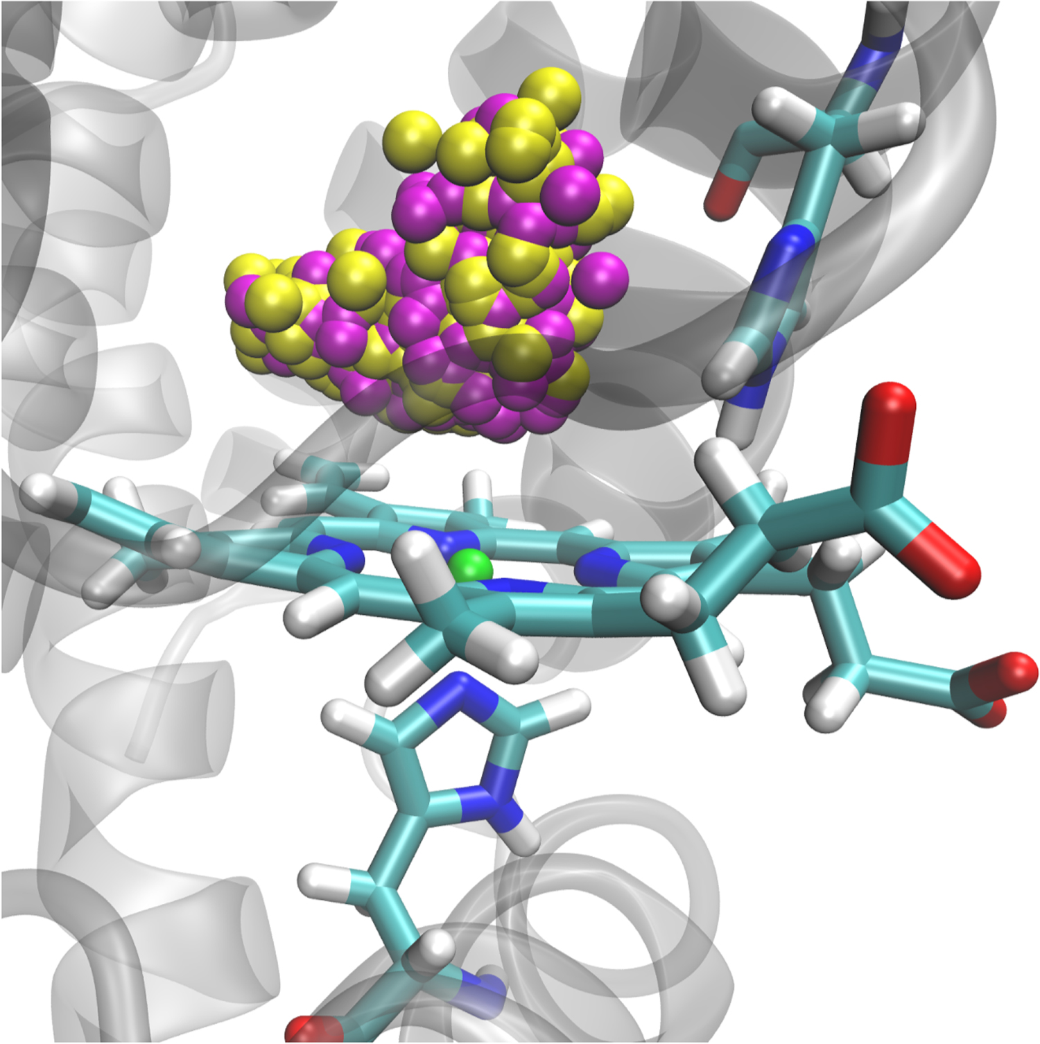
Figure 13. Solvent distribution around FAD for the transition state ensemble from 100 000 transition states sampled from umbrella sampling simulations. The two isosurfaces correspond to fractional occupancies of 10−6 (magenta) and 0.01 (yellow). The maximum value of the fractional occupancy at any point is ∼0.049.
Download figure:
Standard image High-resolution image
The methods discussed in the present work all have their advantages and shortcomings. Depending on the application at hand the methods provide different efficiencies and accuracies and are more or less straightforward to apply. In the following, the three approaches discussed here are compared by looking at them from different perspectives.
- For small gas phase systems such as tri- and tetraatomics, RKHSs, PIPs and NN-based force fields are powerful methods for accurate investigations of their reactive dynamics. Empirical force fields are clearly not intended and suitable for this.
- For medium-sized molecules (up to ∼10 atoms) in the gas phase, reactive MD methods, such as the EVB [49] (not explicitly discussed here or multi state reactive MD), NNs, or suitably parametrized force fields (polarizable or non-polarizable) including multipoles are viable representations. PIPs or RKHSs will eventually become laborious to parametrize and computationally expensive to evaluate.
- Systems with ∼10 atoms in solution can be described by refined FFs and reactive MD simulations. NNs, such as Physnet, would be a very attractive possibility, as they include fluctuating charges by construction. Also, capturing changes in the bond character depending on the chemical environment (see discussion of methylated MA above) is readily possible. However, an open technical question is how to include the effect of the environment in training the NN.
- Finally, for macromolecules in solution, such as proteins, either refined reactive FFs or a combination of RKHS and a FF has shown to provide meaningful ways to extend quantitative, reactive simulations to condensed phase systems. Extending such approaches, akin to mixed QM/MM simulations but treating the reactive part with a NN, may provide even better accuracy.
Multidimensional PESs are a powerful way to run high-quality atomistic simulations for gas- and condensed phase systems. Recent progress concerns the accurate, routine representation of PESs based on RKHSs or PIPs. As an exciting alternative, NN-based PESs have also become available. Despite this progress, extension of these techniques to simulations in solution and multiple dimensions remain a challenge. Attractive future possibilities are simulations which capture the changes in local chemistry or in the atomic charges without the need to explicitly parametrize them as a function of geometry. This is possible with approaches as those used in PhysNet.
Acknowledgments
The authors acknowledge financial support from the Swiss National Science Foundation (NCCR-MUST and Grant No. 200021-7117810) and the University of Basel (to MM). OTU acknowledges funding from the Swiss National Science Foundation (Grant No. P2BSP2_188147).
Data availability statement
The data that support the findings of this study are available from the corresponding author upon reasonable request.