Abstract
We consider the polaron dynamics driven by Froḧlich type, long wavelength dominated electron-phonon interaction at zero temperature, for three different semi-metals: single and bilayer graphene, and semi-Dirac, all grown on polar substrates such as, SiC. Single layer graphene (henceforth called SL graphene), bilayer graphene (henceforth called BL graphene), and semi-Dirac have two dimensional band-structures with point Fermi surfaces in their natural undoped conditions. When these materials are grown on polar substrates, their electrons can interact with the optical phonons (LO) at the surface of the substrates. That gives rise to the possibility of polaron formation in the context of these semi-metals, although they themselves are non-polar. Starting from the Froḧlich type electron-phonon interaction Hamiltonian, perturbation theory is employed to calculate the self energy of the electron due to polaron formation for the three aforementioned systems. The electron self energy, or the polaron energy, calculated analytically for BL graphene, is shown to vary linearly with the electron momentum for small electron momenta. Whereas for ordinary polar crystals (both two and three dimensional), for small electron momentum, the polaron energy is quadratic leading to the mass correction of the electron, for BL graphene the polaron energy disperses linearly, rendering the massive BL graphene electrons effectively massless. Energies for Froḧlich polarons in SL graphene and semi-Dirac on polar substrates, are numerically evaluated. Also, the electron relaxation rate, related to the imaginary part of the analytically continued electron self energy expression, is calculated for the three systems.
Export citation and abstract BibTeX RIS

Original content from this work may be used under the terms of the Creative Commons Attribution 4.0 licence. Any further distribution of this work must maintain attribution to the author(s) and the title of the work, journal citation and DOI.
1. Introduction
There has been extensive studies on the electron-phonon interaction in the context of SL and BL graphene. In those studies, analytical expressions have been derived for the electron-phonon interaction Hamiltonians, considering both the acoustic and the optical modes of phonon-vibrations [1–5]. But in all of them, the electron-phonon interaction isn't dominated by long wavelength phonons.
Long wavelength phonons play an important role in the electron-phonon interaction in polar crystals. In such materials an optical phonon (LO) mode, generated by the oppositely charged ions in an unit cell moving in opposite directions, is accompanied by a dipole moment. The electrostatic potential resulting from such a dipole moment modifies the energy of a nearby electron. This is called the Froḧlich electron-phonon interaction. As it turns out to be the case, in such an interaction the electron-phonon coupling strength, a phonon-wavelength-dependent factor, becomes very strong in the long-wavelength region. In fact, the square of the coupling strength behaves like the electrostatic Coulomb potential in the Fourier space [6], i.e.,  -space,
  being the wave-vector. Like the Coulomb potential, with
  the square of the coupling strength varies as
  and
and  , for a 2-D and a 3-D system respectively [6, 7], becoming very large for small
  or long wavelength. This type of long-wavelength dominated electron-phonon interaction, which is at the heart of Froḧlich interaction, is the cause of polaron formation in polar crystals. Froḧlich type of electron-phonon interaction plays a dominant role at and near the interfaces of hetero-structures [8, 9]. For example, when one considers a sheet of graphene (single or bi-layer) being placed on a polar substrate, such as SiC, the optical phonons at the surface of the latter can couple to the electrons of the former through the above-mentioned interaction. Such a scenario has been considered in [10], in which the primary interest was to study thermodynamic properties like the resistivity of the material. In this paper we will be considering a similar Froḧlich interaction for our study of polaron formation, at zero temperature, in SL, BL graphene and semi-Dirac semi-metals grown on polar substrates.
For the above-mentoned systems, we will calculate the polaron energy for the range of the electron-momentum in which polaron formation is possible. Once the electron momentum goes beyond the range, polaron does not form and the electron loses its energy by means of emitting a phonon. At zero temperature, the initial number of phonons being zero, there is only emission and no absorption of a phonon due to electron phonon interaction. The probability per unit time for the electron transitioning into other states with the emission of phonons, also called the relaxation rate, will be calculated. The organization of the paper is as follows. Having introduced the electron-phonon Froḧlich interaction Hamiltonian, the polaron formation in BL graphene on a polar substrate is considered first. After calculating the polaron energy and the relaxation rate for BL graphene, we next study the polaron dynamics of SL graphene, and finally of semi-Dirac, both materials being considered on polar substrates. In both cases we investigate the polaron energy and the relaxation rate. The reason for treating BL graphene first is that, unlike SL graphene and semi-Dirac, it has been possible to obtain an analytical result for the polaron energy of BL graphene for small values of the electron momentum. This analytical result clearly shows that there exists a linear relationship between the polaron energy and the corresponding momentum, when the momentum is small, making the BL graphene polaron massless.
2. Froḧlich type electron-phonon interaction Hamiltonian
We briefly explained the origin of the Froḧlich interaction in the introduction section. In the following, we will first write the Hamiltonian of such an interaction. We will then explain various components of the Hamiltonian. The Hamiltonian is given by [10].

In equation (1), the Bosonic operators  and
and  are the annihilation and the creation operator of an optical phonon (LO) at the surface of the polar substrate, for the phonon wave-vectors
  and
and  respectively. They satisfy the standard Bosonic commutation relations, viz.,
 ![$[{b}_{\vec{k}},{b}_{\vec{q}}^{\dagger }]={\delta }_{\vec{k},\vec{q}}$](https://content.cld.iop.org/journals/2399-6528/5/1/015009/revision3/jpcoabd69aieqn11.gif) , and
, and ![$[{b}_{\vec{k}},{b}_{\vec{q}}]=0$](https://content.cld.iop.org/journals/2399-6528/5/1/015009/revision3/jpcoabd69aieqn12.gif) . We will assume, as is customary, a LO phonon to be non-dispersive.
. We will assume, as is customary, a LO phonon to be non-dispersive.
 in equation (1) is the Fourier transform of the density operator Ψ†(x)Ψ(x) for the electrons [11], where Ψ(x) is the second quantized version of the real space eigen-function for the 'unperturbed' Hamiltonian of a semi-metal considered in the paper. The Hamiltonians being matrices, Ψ(x) is a spinor (associated with the pseudospin dregree of freedom of the systems). Ψ(x) can be expressed as
  , A, the normalizing factor, being the area of the primitive cell of the semi-metal.
  is the momentum-space eigen-spinor (corresponding to the wave-vector
  ) of the semi-metal Hamiltonian, and the Fermionic operator
  is the annihilation operator of an electron of wave-vector
  . The standard Fermionic anti-commutation relations, viz.,
  , and
, and  , are obeyed.
We have intentionally omitted the band and real spin indices in the expression for Ψ(x). The band indices are omitted, since, for Froḧlich interaction, inter-band terms are absent [12]. As is standard for the electron self energy calculation in such an interaction, the electron states, including the initial, the final and all the intermediate states in the perturbation expansion of energy are conduction band states. The spin index in Ψ(x) is also suppressed to keep notations simple. The spin degeneracy factor gs is included in the final expressions for polaron energy and the relaxation rate [7].
Using the above-mentioned expression for Ψ(x),  , the Fourier transform of the electron density function Ψ†(x)Ψ(x), assumes the following form

Next, following Ref. [10], the long-wavelength (small  ) dominated term
  in equation (1) is given by
  , where q is
  . For small q,
  in the above goes as
  , just like an electrostatic potential in two dimensions. g in
  is a constant specific to a polar substrate and D is the average distance between the substrate and the semi-metal under consideration. g is given by [12],

where  ,
,  s
and ∞ being the static and high frequency permittivities respectively of the substrate. ωs
is the frequency of the optical phonons (LO) at the surface of the polar substrate; e is the charge of an electron and As
, the area of the primitive cell (inversely related to the area of the phonon Brillouin zone). Quantities like
s
and ∞ being the static and high frequency permittivities respectively of the substrate. ωs
is the frequency of the optical phonons (LO) at the surface of the polar substrate; e is the charge of an electron and As
, the area of the primitive cell (inversely related to the area of the phonon Brillouin zone). Quantities like  and ωs
are substrate specific. As an example [10], for SiC, ωs
and
and ωs
are substrate specific. As an example [10], for SiC, ωs
and  are 116 meV and .05 respectively. The value of
  follows from s
, and ∞, for SiC, being 9.7 and 6.5 respectively.
follows from s
, and ∞, for SiC, being 9.7 and 6.5 respectively.
Finally, using equation (2) for  and the above-mentioned expression for
  in equation (1), one obtains

where g is given by equation (3). Equation (4) is the long-wavelength dominated Froḧlich interaction Hamiltonian that will be used for all our subsequent calculations for all the three systems. It is seen from equation (4) that this Hamiltonian has both the Fermionic and the Bosonic operators multiplying each other, which represents the electron-phonon interaction.
3. Deriving the general polaron energy expression for the semi-metals
In this section, we will obtain the energy correction for an electron of wave-vector  in the conduction band of the semi-metal under consideration, due to the interaction Hamiltonian given by equation (4), the initial and the final wave-vector
  of the electron remaining unchanged. Since there are no phonons in the initial and the final state, and the interaction Hamiltonian given by equation (4) changes the number of phonons, the first order energy correction will be zero. The first non-vanishing electron energy correction will arise from the second order perturbation expression for the energy. The self energy (ΔE) of the electron at this order is given as follows [7]:

In equation (5),  is the initial as well as the final state, which has only one electron of wave-vector
  and no phonons. This state in the second quantized notation can be written as,
  , where
  corresponds to the 'vacuum'. ['vacuum' refers to the absence of the electron of interest, as well as the absence of any phonons]. Perturbation theory demands that the intermediate state
  in equation (5) can be anything but the initial state
  . But we won't need to mention that restriction explicitly in equation (5) since the matrix element
  is 0.
is 0.
Denoting the energy of the 'free' electron in the initial state as  , E0 in equation (5) can be written as
  . The intermediate state
  can be written as
  , where
  stands for the wave-vector of the phonon, and
  stands for the wave-vector of the electron. In the second quantized notation, the intermediate state
  can be expressed as
  ,
,  and
and  corresponding to the phonon and electron creation operators respectively. ∑n
in equation (5) is actually
corresponding to the phonon and electron creation operators respectively. ∑n
in equation (5) is actually  .
.
En
, the energy of the intermediate state  , can be written as the sum of the energy of the 'free' electron (denoted as
  ) and that of the phonon with wave-vector
  . The phonon being a LO phonon, has a momentum-independent constant frequency ωs
, and energy ℏωs
. Hence En
can be written as
. The phonon being a LO phonon, has a momentum-independent constant frequency ωs
, and energy ℏωs
. Hence En
can be written as  . Finally, using equation (4) for the Hamiltonian, and the standard commutation (anticommutation) relations for Bosonic (Fermionic) operators, we obtain from equation (5)

The factor  in the numerator of equation (6) describes the overlap of the spinors, also called the overlap factor. The spin degeneracy factor gs
has been incorporated in equation (6) to make the energy expression complete.
in the numerator of equation (6) describes the overlap of the spinors, also called the overlap factor. The spin degeneracy factor gs
has been incorporated in equation (6) to make the energy expression complete.
The following is a Feynman diagram showing a second-order electron-phonon interaction, in which a phonon, shown as a wavy line in the diagram, is emitted and then re-absorbed. The solid lines in the diagram represent electrons. In the Feynman diagram, despite the interaction, the electron's initial and the final states are the same having the same wave-vector  . At each node of the Feynman diagram, the momentum conservation law is obeyed as indicated in the diagram. The Feynman diagram serves as a visual aid. As for the polaron energy calculation, equation (6) is used directly.
4. General expression for the relaxation rate
When an electron in the semi-metal conduction band is 'too energetic', the polaron formation is not possible. The electron then loses its energy by making a transition from its current state to another accompanied with the emission of a phonon. The corresponding transition probability per unit time ( ), or the relaxation rate, is twice the imaginary part of the polaron energy expression as given by equation (6) divided by ħ, after having analytically continued the denominator in the expression to the complex plane [7] and is expressed as

The argument of the δ function in equation (7) is also what appears in the denominator of equation (6). It will be shown that the argument  of the δ function can be 0, and hence
  , non-vanishing, provided the magnitude of the electron momentum
  crosses a limit. This limit, or the cut-off momentum, is dependent on the conduction band energy momentum dispersion relation of the semi-metal under consideration and hence different for different semi-metals. As long as the electron momentum stays below that cut-off, a polaron will be formed.
5. Analytical derivation of the polaron energy for BL-graphene on a polar substrate
In this section we will compute the polaron energy as given by equation (6) for a BL graphene-electron. The low energy electronic structure of BL graphene, in its undoped condition, consists of two parabolic bands touching each other at a point Fermi surface. The Hamiltonian of BL graphene in the momentum space (ℏpx , ℏpy ) is given by:
with the eigen-energies  , the + sign corresponding to the conduction band eigenspinor

where  .
.
The overlap factor in equation (6) can be calculated using the spinors given by equation (8), to yield the following expression (The details of the calculation is shown in appendix A).

where γ and ϕ are the angles that the wave-vectors  and
and  make w.r.t the x axis respectively. The magnitudes of the vectors
  and
and  are denoted by l and q respectively. A new angular variable
  can now be introduced and
  in equation (6) can be replaced as
  . As
is the same as the one appearing in equation (3). Also, BL graphene conduction band energies
. As
is the same as the one appearing in equation (3). Also, BL graphene conduction band energies  and
and  are used in equation (6).
The system-parameters m and ωs
, along with ℏ, can be combined to yield the natural length scale  . It can be used to define the following dimensionless quantities:
  and
and  . We call them 'dimensionless electron momenta' or 'DEM's, which are essentially momentum variables in units of
  . We replace
  and
and  in equation (6), wherever they appear, by these dimensionless variables. g is given by equation (3). Putting all the above-mentioned pieces together in equation (6), we obtain the following equation for the polaron energy for BL graphene

where α is the Froḧlich oupling constant, as given by  .
.  in the above expressions is a dimensionless quantity given by
  . We will consider the specific case of BL graphene grown on SiC substrate, for which ωs
= 116 meV,
. We will consider the specific case of BL graphene grown on SiC substrate, for which ωs
= 116 meV,  and D, the average distance between the BL graphene sheet and the polar substrate, is 6 Å as per [10]. These values along with the standard values of electron-mass m and ℏ yield α ≈ 1.5 and
  . Other values of
  can be obtained for other substrates, but as long as they are of the same order of magnitude, the essential physics will change little. For all our calculations involving BL graphene we will use
  .
.
Next, we will evaluate equation (10) analytically for small  , corresponding to small electron momentum. To that end the factor
  appearing in equation (10) is first simplified to give
  . Next, since
  , it is possible to write
  , which is true for all
  and
and  . Hence,
  can be Taylor-expanded as follows [11].
Using equation (11) in equation (10) and carrying out integrations, we obtain the following expression for ΔEBLG (The details of the calculation is given in the appendix B)

Using  for
for  in equation (12), we obtain

In equation (13) there is a constant term and a term linear in the DEM. In figure 1 the absolute value of the polaron energy ΔEBLG given by equation (13) is plotted (in the units of αℏωs
) w.r.t the DEM  . In the same figure the absolute value of ΔEBLG, evaluated numerically by using equation (10) directly, is also plotted w.r.t
  for comparison.

Figure 1. Absolute Value of Polaron Energy (in the units of αℏωs
) Versus Dimensionless Electron Momentum (DEM)  for BL Graphene for Small
  .
.
Download figure:
Standard image High-resolution imageIt can be seen from figure 1 that the analytical result agrees with the numerical result as long as  isn't too large.
Writing the DEM in terms of actual electron momentum  , one obtains the following energy momentum relationship from equation (13).

where  is the magnitude of the electron momentum
  . Equation (14) explicitly shows that the BL graphene polaron energy disperses linearly with
  . Equation (14) is valid provided
  is small. Now, to get the total energy, the unperturbed original energy of the BL graphene conduction-band electron, which varies as
  , needs to be added to ΔEBLG. But, for small
  , it is less significant than the term linear in
  in ΔEBLG. Hence, it is concluded that BL graphene polarons behave as massless quasiparticles for small electron momenta. This is the key result of this paper. The coefficient
  , in front of the electron momentum in equation (14), is the magnitude of the slope of the linear energy-momentum graph, had equation (14) been plotted graphically, and has the dimension of velocity. This is the velocity of a massless polaron in BL graphene. It is noted that the polaron velocity does not depend on
  , and hence is independent of the exact distance between the BL graphene sheet and the polar substrate. For
  substrate, the numerical estimate of the BL graphene polaron velocity is
  .
.
The linear energy momentum dispersion of BL graphene polarons can experimentally be verified through Angle Resolved Photoemission Spectroscopy (ARPES) [13]. The presence of the polaron quasi-particle can be ascertained by looking for the signature peak-dip-hump(PDH) structure–consisting of an actual peak accompanied by a smaller satellite one—in the experimentally obtained spectral function  , where
  , and are the momentum and the energy variables respectively. For a given
  , the spectral function achieves its maximum at the polaron quasiparticle energy. Thus the quasiparticle energies, experimentally obtained through ARPES, can be plotted as a function of the momenta. The plot should look linear. Comparing the slope of that plot with the theoretically predicted polaron velocity
  of equation (14), one can extract the Froḧlich coupling constant α, since ωs
and m are known quantities in the expression of the velocity. Once α is ascertained, the experimental energy momentum plot can be compared against the theoretical prediction of equation (14).
of equation (14), one can extract the Froḧlich coupling constant α, since ωs
and m are known quantities in the expression of the velocity. Once α is ascertained, the experimental energy momentum plot can be compared against the theoretical prediction of equation (14).
Using ARPES, The Froḧlich coupling constant α can also be extracted in a slightly different way than what is described above, as follows. One can determine α by measuring the strength of the peak of the spectral function  at the electron momentum
  and = the polaron energy, following an approach similar to that outlined in [12]. The quasiparticle peak-strength Z of the spectral function
  is related to the self energy function(defined as
  ) through the relationship
  , where the self energy
  is given by an expression similar to the one in equation (6) with the energy variable in the place of
  , and everything else remaining the same. We calculated Z for BL graphene using the above-mentioned expression and found Z ≈ 1 − .74α. In deriving this expression, we used ΔEBLG(p = 0) = − .27αℏωs
, as is obtained from equation (14), setting
, and everything else remaining the same. We calculated Z for BL graphene using the above-mentioned expression and found Z ≈ 1 − .74α. In deriving this expression, we used ΔEBLG(p = 0) = − .27αℏωs
, as is obtained from equation (14), setting  . Equating the theoretical value of Z = 1 − .74α to the experimentally measured strength of the quasiparticle peak of the ARPES spectral function at
  , one can ascertain the value of the coupling constant α.
Cyclotron resonance experiment can also be deployed to extract α. Following the same approach as that of [14], the Landau like energy levels for the BL graphene polarons in a magnetic field can be obtained by studying the photoconductive response resonance-peaks, and recording the energy and the magnetic field values, where those peaks occur. That will give a relationship between the Landau like energy levels of the polaron and the magnetic field. By comparing this with the corresponding theoretical expression, in which the parameter α will evidently show up, one can extract α. But for that one would first need to study theoretically the Landau levels of BL graphene polarons in the presence of a magnetic field. This is a possible future direction of the current work.
Another way to use the magnetic field to calculate α is by measuring the cyclotron mass through studying Shubnikov-de Haas oscillations (SdHO) [15]. The cyclotron mass can then be set equal to the theoretical expression [16] for the cylotron mass, given by  , where A() is the area of the cyclotron orbit in the momentum space for a given particle energy . But obtaining an expression for cyclotron mass for the BL graphene polaron needs further theoretical work and can be undertaken as a follow-up of the current work.
6. The relaxation rate for the BL graphene electron
The relaxation rate for the BL graphene electron can be obtained from equation (7) by replacing  and
and  by appropriate conduction band energy expressions for BL graphene. Also, having replaced
  in equation (7) by equation (9), and g in equation (7) by equation (3), one obtains the following relaxation rate for BL graphene in terms of DEMs
  and
and  .
.

The details of the evaluation of equation (15) are given in appendix D. It can be shown with a little algebra that the argument of the δ function,  , is always greater than 0, and hence never 0, regardless of the values of
  , and the angle
  between
  and
and  , as long as
  . Hence to have a non-zero relaxation rate, we must have
  . The cut-off momentum, introduced before, is
  , in terms of DEM for BL graphene. Polaron quasiparticle forms when
  . When
  , no polarons are formed and the electron relaxation rate is given by equation (15).
In equation (D3), the relaxation rate  has been evaluated as function of the DEM
  . Using the relationship between BL graphene electron energy and
  , e.g.,
  , the relaxation rate can be expressed as a function of the electron energy(in units of ℏωs
). In figure 2 the relaxation rate is plotted (in units of α
ωs
) as a function of the electron energy (in units of ℏωs
), for an appropriate energy range, viz.,
, the relaxation rate can be expressed as a function of the electron energy(in units of ℏωs
). In figure 2 the relaxation rate is plotted (in units of α
ωs
) as a function of the electron energy (in units of ℏωs
), for an appropriate energy range, viz.,  (corresponding to
  ). From the figure, the maximum value of the relaxation rate is ascertained at approximately .6α
ωs
. For BL graphene on the polar substrate SiC, α and ωs
are 1.5 and 116 meV respectively. This puts the maximum value of the relaxation rate at approximately 160 GHz.
). From the figure, the maximum value of the relaxation rate is ascertained at approximately .6α
ωs
. For BL graphene on the polar substrate SiC, α and ωs
are 1.5 and 116 meV respectively. This puts the maximum value of the relaxation rate at approximately 160 GHz.

Figure 2. Relaxation Rate (in units of α ωs ) Versus Electron Energy (in units of ℏωs ) for BL Graphene.
Download figure:
Standard image High-resolution imageIt is seen from figure 2 that the relaxation rate for BL graphene increases, peaks at a certain value of the electron energy and then falls off as energy further increases. This is different from the electron relaxation rate in conventional two dimensional polar crystals, which decreases monotonically to zero with the increase of electron energy.(This can be shown with the help of a calculation similar to the one carried out in [7].) The relaxation rate for BL graphene can be measured with the help of pump-probe spectroscopy as outlined in [17]. The relaxation rate can be ascertained for various polaron energies by measuring probe transmissions as a function of the time delay between the pump and the probe. The probe transmission can then be fitted with an exponentially decaying function, from which the relaxation rate can be extracted. The experimentally obtained relaxation rate can then be compared with figure 2.
7. Numerical evaluation of the polaron energy and the relaxation rate for SL graphene
In this section, for SL graphene on a polar substrate, we will compute the polaron energy and the relaxation rate. One-atom thick SL graphene has drawn a lot of attention since its experimental realization by Novoselov and Geim because of its low energy linear dispersion with point Fermi surface. SL graphene Hamiltonian is given by  . vF
is the Fermi velocity, and
. vF
is the Fermi velocity, and  is the electron wave-vector. The conduction band electron energy of
  is given by
  and the corresponding electron eigen-spinor, by

where  .
.
In order to obtain polaron energy for SL graphene, the electron eigen-spinors  and
and  in equation (6) are substituted by appropriate SL graphene eigen-spinors. This can be accomplished by replacing
  in equation (16) by
  and
and  respectively. Also, in equation (6), the 'non-interacting' electron energies
  and
and  are given by the SL graphene electron energies
  and
and  respectively.
  in equation (6) for SL graphene can be shown to be equal to
 ![$\tfrac{1}{2}\left(1+\tfrac{1}{| \vec{l}-\vec{q}| }\left[l-\tfrac{\vec{l}\cdot \vec{q}}{| \vec{l}| }\right]\right)$](https://content.cld.iop.org/journals/2399-6528/5/1/015009/revision3/jpcoabd69aieqn166.gif) with the help of the SL graphene eigen-spinors. As we did in case of BL graphene, we replace
with the help of the SL graphene eigen-spinors. As we did in case of BL graphene, we replace  by
by  , where
  is the angle between
  and
and  . The natural length-scale for the SL graphene-polar crystal assembly is
  , which can be used to introduce the dimensionless momenta (DEMs)
  , and
, and  . DEM for SL graphene is essentially the electron momentum in the units of
  .
.
Finally replacing g by equation (3) and inserting the spin degeneracy factor gs
, equation (6) assumes the following form in terms of the dimensionless variables  and
and  , and the angle
  between them.

where  , and
, and  , a dimensionless constant. As was done in case of BL graphene, we consider the SL graphene on SiC substrate. Following [10], using ωs
= 116 meV,
, a dimensionless constant. As was done in case of BL graphene, we consider the SL graphene on SiC substrate. Following [10], using ωs
= 116 meV,  , D = 4Å and vF
= 106 m s−1, we obtain α = .01, and
, D = 4Å and vF
= 106 m s−1, we obtain α = .01, and  . We will recourse to numerical methods for evaluating equation (17).
The relaxation rate for SL graphene is calculated from equation (7) by replacing g by equation (3), and  ,
,  and
and  by suitable expressions for SL graphene. The relaxation rate, thus evaluated and expressed in terms of DEMs
  and
and  , assumes the following form.
The details of the evaluation of the relaxation rate as given by equation (18) is included in appendix E. The argument of the δ function,  , is always greater than 0, and hence never 0, regardless of the values of
  and
and  as long as
  . Hence to have a non-zero relaxation rate, we must have
  . Polaron quasiparticle forms when
  . Figure 3 shows the plots of the absolute value of the polaron energy and the relaxation rate of SL graphene w.r.t to DEM
  . The polaron energy and the relaxation rate are evaluated using equations (17) and equation (E3) respectively. Now, the DEM
  for SL graphene can also be thought of as the energy variable in the units of ℏωs
. This can clearly be seen by writing SL graphene electron energy
for SL graphene can also be thought of as the energy variable in the units of ℏωs
. This can clearly be seen by writing SL graphene electron energy  as
as  , by employing the definition of
  . Hence the relaxation rate for SL graphene electron versus the DEM
  plot is the same as the relaxation rate vs the electron energy plot, the energy variable being expressed in the units of ℏωs
.
plot is the same as the relaxation rate vs the electron energy plot, the energy variable being expressed in the units of ℏωs
.

Figure 3. Above: Absolute Value of Polaron Energy (in units of αℏωs
) Versus Dimensionless Electron Momentum (DEM)  for SL Graphene Below: Relaxation Rate (in units of α
ωs
) Versus Energy (in units of ℏωs
) for SL Graphene.
for SL Graphene Below: Relaxation Rate (in units of α
ωs
) Versus Energy (in units of ℏωs
) for SL Graphene.
Download figure:
Standard image High-resolution imageFrom figure 3 it is seen that the polaron energy for SL graphene changes fairly linearly with dimensionless electron momentum (DEM), not only for small DEM, but throughout the allowed range of the DEM. This is in line with the linear energy-momentum dispersion of 'non-interacting' SL graphene electrons. From figure 3, and making use of the definition of DEM, the equation for SL graphene polaron energy can be estimated as  where
where  is the magnitude of the electron momentum
  . From the expression of
  , the magnitude of the 'velocity-factor' multiplying the electron momentum is
  and is approximately
  , for
, for  . This is of the same order of magnitude as the BL graphene polaron velocity for small electron momenta. But, for SL graphene, this is not the polaron velocity. To obtain the polaron velocity, one needs to add the unperturbed electron conduction band energy
  , also linear in the electron momentum, to the polaron energy
  , making the total electron energy
  (upto a constant term). The constant factor
  in front of the electron momentum in the total energy-momentum relationship is the polaron velocity. It indicates that the velocity of the SL graphene electrons is about one tenth lesser than its usual value
  due to the polaronic effect. In other words, the polaronic effect makes SL graphene electrons 'slower'. As for the SL graphene electron relaxation rate plotted in figure 3, it initially goes up with the increase in electron energy, and then flattens. This is quite different from the relaxation rate pattern of BL graphene, as given by figure 2. Unlike SL graphene, the relaxation rate for BL graphene falls off for large values of the electron energy. The maximum value of the SL graphene relaxation rate in figure 3 is
  50 (in units of α
ωs
). For SL graphene on the polar substrate SiC, α and ωs
are .01 and 116meV respectively. This puts the maximum value of the relaxation rate at approximately 85 GHz, about half of the corresponding quantity for the BL graphene.
50 (in units of α
ωs
). For SL graphene on the polar substrate SiC, α and ωs
are .01 and 116meV respectively. This puts the maximum value of the relaxation rate at approximately 85 GHz, about half of the corresponding quantity for the BL graphene.
Whereas the relaxation rate as a function of energy for SL graphene is in stark contrast with the relaxation rate as a function of energy for BL graphene, the polaron energy of SL graphene shares a striking similarity with the small-momentum polaron energy of BL graphene. Despite the fact that that SL and BL graphene have very different electronic energy momentum dispersion relationship in the absence of electron-phonon interaction, the two systems behave rather similarly (both having linear energy-momentum dispersion) so far as the polaron-energy in the small momentum region is concerned. Incidentally it can be mentioned that the relaxation rate for the SL graphene polarons is quite similar to the relaxation rate for polarons in conventional three dimensional polar crystals with quadratically dispersing electrons [7].
The graphene polaron energy-momentum can be experimentally verified by ARPES measurement just like BL graphene. The strength of the spectral function peak will give useful information about the Froḧlich coupling constant α. The strength of the peak is equal to the Z factor, as was mentioned in the case of BL graphene. Z is related to the self energy function  , and
, and  being the energy and the momentum variables respectively) through the relationship
  . Using ΔESLG(P = 0) = − 11αℏωs
, we evaluated Z for SL graphene to be Z = 1 − 4.7α. Equating this theoretical value of Z to the experimentally measured strength of the quasiparticle peak of the spectral function at
. Using ΔESLG(P = 0) = − 11αℏωs
, we evaluated Z for SL graphene to be Z = 1 − 4.7α. Equating this theoretical value of Z to the experimentally measured strength of the quasiparticle peak of the spectral function at  , one can calculate the value of the coupling constant α.
The cyclotron resonance can give us useful information about the Froḧlich coupling constant α too, in a similar vein along BL graphene. As in BL graphene, the Landau like energy levels of the SL graphene polaron, in the presence of a magnetic field, need to be calculated theoretically, before one can compare it to the experimental data and extract α from it. (Landau levels of SL graphene in the presence of a magnetic field has been studied [16, 18, 19], but the Landau levels of SL graphene polarons is novel.) Another way to extract α, for SL graphene, is to calculate the cyclotron mass for the SL graphene polaron and compare it to the mass experimentally obtained by de Van Has Alphen effect. Both can be considered as the future directions for the current work.
8. Polaron energy and relaxation rate for semi-Dirac on a polar substrate
Semi-Dirac materials drew research interest in recent years due to is anisotropic, exotic electronic band-structure dispersing linearly in one direction and quadratically in the orthogonal direction in the Brillouin zone [20–25]. It was first discovered computationally in oxide heterostructures [26]. We consider semi-Dirac, like SL and BL graphene, to be grown on a polar substrate. The resulting polaron-dynamics is investigated. As was discovered in [26], the interfaces of  heterostructure, in which semi-Dirac dispersion was observed, are non-polar. This justifies the treatment of semi-Dirac, for the purpose of this paper, in the same footing as non-polar materials like SL and BL graphene.
The energy momentum dispersion relation for a semi-Dirac electron is given by  , the positive and the negative signs corresponding to the conduction and the valence bands respectively. m is the mass-parameter and vF
is the velocity parameter. px
and py
are the electron wave-vectors along two special directions in the Brillouin zone, viz., x and y. Along the x direction, semi-Dirac energy disperses quadratically like an ordinary electron. Hence x is called the non-relativistic direction. Along the y direction, semi-Dirac energy disperses linearly, like SL graphene. Hence y is called the relativistic direction.
, the positive and the negative signs corresponding to the conduction and the valence bands respectively. m is the mass-parameter and vF
is the velocity parameter. px
and py
are the electron wave-vectors along two special directions in the Brillouin zone, viz., x and y. Along the x direction, semi-Dirac energy disperses quadratically like an ordinary electron. Hence x is called the non-relativistic direction. Along the y direction, semi-Dirac energy disperses linearly, like SL graphene. Hence y is called the relativistic direction.
The above-mentioned energy-momentum relationship for semi-Dirac can be derived from more than one Hamiltonian related to each other by unitary transformations. To get the essential physics, keeping the computations as simple as possible, we will use the following form of the 'non-interacting' semi-Dirac Hamiltonian as given by  . The electron eigenstate of
  is given by

where,

Next, to compute the polaron energy for semi-Dirac, the spinors  and
and  in equation (6) are replaced by the semi-Dirac spinors, as given by equation (19), using
  and
and  for
for  respectively. The conduction band energies
  and
and  in equation (6) for semi-Dirac are given by
  and
and  respectively. For semi-Dirac, there are two length scales, e.g.,
  , and
, and  . They are used to convert the x and the y components of the wave-vectors into dimensionless momenta variables (DEMs) differently. For the wave-vector
  we define the DEMs
  , and
, and  , and an exactly similar set of DEMs for the wave-vector
  .
.
Finally, using the standard replacements of g by equation (3), and  by
by  in equation (6), one obtains the semi-Dirac polaron energy as

where W and R are given by


In equation (21), α is the Froḧlich constant given by  . For SIC substrate having the surface phonon frequency ωS
= 116 meV and
. For SIC substrate having the surface phonon frequency ωS
= 116 meV and  , α ≈ 1.5. κ is a dimensionless constant given by
  . κ ≈ 49 for SiC substrate.
  is a dimensionless quantity given by
  . For semi-Dirac, an average value of D can be taken to be about 15 Å for the following reason. As per [26], in
  hetero-structure, the semi-Dirac band-structure sports the signature of the Vanadium atoms, which in the real space are located above 5 layers of TiO2 of about a total of 1.5 nm thickness. Hence, if
  layered structure is grown on a polar substrate, it is not unreasonable to assume that the semi-Dirac electrons will be separated from the substrate by at least 1.5 nm thick TiO2 layers, creating an average distance D = 15 Å between the polar substrate and the electron. For SiC substrate, using D = 15 Å, one obtains
  .
.
Next, before evaluating equation (21) numerically, we will obtain an expression for the relaxation rate of semi-Dirac electrons. In the relaxation rate formula given by equation (7), we replace g by equation (3) as usual;  and
and  by appropriate semi-Dirac energies; and
  and
and  by appropriate semi-Dirac eigen-spinors of the form as given by equation (19). Finally, employing the definitions of DEMs
  and
and  , the relaxation rate, as per equation (7) takes the following form for the semi-Dirac polaron.

where W and R are given by equation (22).
Like in the previous two cases, studying the argument of the δ function in the expression for the relaxation rate gives information about the cut-off momentum. From equation (23), the argument R, as given by equation (22b
), of the δ function is guaranteed to be greater than 0, if  is less than 1. Defining γ as the angle that DEM
  makes w.r.t the x-axis, and writing
  and
and  ,
,  can be expressed as
  . It can be shown with a little algebra that the above-mentioned quantity is less than 1, if
  satisfies the following criterion.

Inequality (24) sets an upper cut-off value for DEM  , such that for DEMs having values less than that cut-off value, the argument R of the δ function in equation (23) can never be 0, and hence resulting in zero relaxation rate. This corresponds to the polaron formation in the context of semi-Dirac. Once the DEM crosses this limit, there is no polaron formation and the electron relaxation rate is given by equation (23).
It is seen from inequality (24) that the cut-off DEM for the semi-Dirac system is a function of the angle γ that  makes with x-axis. This is due to the anisotropic nature of the energy-momentum relation of a semi-Dirac system. The upper-bound of
  , i.e., the right side of the inequality (24), can be proven to vary from 1 to
  . The upper-bound of
  assumes the value
  when γ = 0, corresponding to the electron momentum being in the x or the 'non-relativistic' direction. The upper-bound of
  is 1 when
  , corresponding to the electron momentum being in the y or the 'relativistic' direction. For any intermediate angle, the upper-bound is in between these two limits. There is no need to consider γ beyond
  , since in inequality (24) only the even powers of quantities like
  , and
, and  appear. In figure 4, the angular dependence of the upper bound of the DEM
  for semi-Dirac is plotted against γ. It can be seen from the figure that the upper-bound of the DEM varies monotonically with angle γ between the two extreme limits 1 and
  , as mentioned before.

Figure 4. Upper Cutoff of the Dimensionless Electron Momentum (DEM)  Versus Angle γ for Semi-Dirac.
Download figure:
Standard image High-resolution imageNext, the absolute value of the polaron energy as given by equation (21) for the semi-Dirac system, is plotted, in the units of αℏωs
in figure 5 for small DEMs. It is seen that so far as the semi-Dirac polaron energy goes, there is a stark difference between the 'non-relativistic' direction corresponding to γ = 0, and any other direction. There is a gap in the energy values between the non-relativistic direction and other directions when the DEM  is zero. For all the directions excepting the 'non-relativistic' one, the polaron energies tend to the same unique value when the DEM
  approaches the value 0. This exotic limiting behavior of polaron energy puts the semi-Dirac system in a very different category from other materials including SL and BL graphene.

Figure 5. Absolute Value of the Energy (in the units of αℏωs
)Vs Dimensionless Electron Momentum (DEM)  for Various γs for Semi-Dirac.
Download figure:
Standard image High-resolution imageNext, we discuss whether the semi-Dirac polaron energy disperses linearly with DEM. Unlike in BL and SL graphene, DEM in semi-Dirac is generally not proportional to the electron momentum excepting when the electron momentum has either only the x-component or only the y-component, i.e., the electron moves either in the 'non-relativistic' or in the 'relativistic' direction. From the plot of figure 5, the polaron energies in these two special directions, corresponding to γ = 0, and  , appear to not be linear for small momentum. This behavior is a departure from the linear nature of the polaron energy-momentum dispersion in both the SL and the BL graphene for small momentum. This shows that semi-Dirac, although resembling SL and the BL graphene along two special directions from the point of view of the non-interacting electron-energy, behaves very differently from those materials so far as its polaron energies in those directions are concerned.
In figure 6, the relaxation rate for semi-Dirac electrons, given by equation (23) and further simplified in appendix F, is plotted, for various γs (in the units of α
ωs
), as a function of semi-Dirac electron energy (in the units of ℏωs
), which can be expressed as  . In all the plots it has been maintained that
  , thereby ensuring that inequality (24) is satisfied for all the values of γ, which is quintessential for the relaxation rate to be non-zero. From figure 6 it can be seen that the relaxation rate changes with electron energy differently for different γs. In figure 6 the plot of the relaxation rate for γ = 0 (the non-relativistic direction) vs energy is similar to the plot of the BL graphene relaxation rate vs energy, as given by figure 2. This behavior is commensurate with the fact that the semi-Dirac energy momentum dispersion of non-interacting electrons along γ = 0 reduces to that of BL graphene.

Figure 6. Relaxation Rate (in the Units of α ωs ) Vs Electron Energy (in the Units of ℏωs ) for Various γs for Semi-Dirac.
Download figure:
Standard image High-resolution imageNext we compare the plot of the relaxation rate vs energy for  in figure 6 with the relaxation rate versus energy plot for SL graphene, given by figure 3. This is of interest since the semi-Dirac energy momentum dispersion of non-interacting electrons along
  reduces to that of SL graphene. It is seen that the relaxation rate stays more or less constant with energy for semi-Dirac along
  , whereas for SL graphene the relaxation rate, after initially increasing with energy, flattens out. It is claimed that the aforementioned two plots are nonetheless similar. The absence of the initial increase of the relaxation rate in case of semi-Dirac is attributed to the large value of κ used in the numerical evaluation of equation (23). It has been checked that with smaller κ's one can actually observe the relaxation rate increasing before flattening out in a similar vein along the SL graphene relaxation rate. Hence, so far as the relaxation rate goes, semi-Dirac behaves as BL graphene or SL graphene depending on whether the electron-momentum is aligned along the non-relativistic or the relativistic direction. This is commensurate with the fact that the semi-Dirac energy momentum dispersion of non-interacting electrons reduces to that of BL graphene (SL graphene) along non-relativistic (relativistic) direction. In figure 6, as for the values of γ which are in between 0 and
  , the relaxation rate vs energy plots are similar to that of γ = 0 in the sense that the relaxation rate falls off for sufficiently large values of energy. Hence the relativistic direction (
 ) stands out w.r.t the relaxation rate of the semi-Dirac system.
Experimental verification of the energy momentum dispersion semi-Dirac polarons can be accomplished through SX(Soft-x-ray)-ARPES measurement as described in [13]. Using soft x-ray will be particularly advantageous for the semi-Dirac system. Due to the enhanced probing distance of the soft (longer wavelength) x-ray, the TiO2/VO2 layers of the semi-Dirac system can be probed deeply for detecting polarons. Like BL and SL graphene, one would look for the peak-dip-hump(PDH) pattern in the spectral function for a given momentum. To compare the experimentally obtained polaron energy momentum relationship with figure 5, one has to first convert the Brillouin zone momenta into the DEMs by using appropriate scalings, which are different for two mutually orthogonal directions in the Brillouin zone. That can readily be done right after obtaining the resonance peaks in the spectral function for various values of the quasiparticle energy and electron momenta along different directions in the Brillouin zone.
The cyclotron resonance experiment for the semi-Dirac will not be very helpful, so far as investigating the Froḧlich coupling constant is concerned. It is because the Landau-like energy levels of the semi-Dirac polarons on a polar substrate in the presence of the magnetic field may not have a particularly simple theoretical expression, not to mention that obtaining such a theoretical expression can be quite challenging. From the measured Landau like energy level versus the magnetic field curve, extracting the α parameter would be rather messy. For a similar reason, the cyclotron mass measurement of the semi-Dirac system might not be a very useful technique either. SX-ARPES measurement seems to be the most suitable method for studying the polaron dynamics of the semi-Dirac system.
9. Summary
In this paper Froḧlich polaron dynamics for the three two dimensional semi-metals, viz., BL and SL graphene, and semi-Dirac has been studied. The materials are assumed to be grown on polar substrates. Both the polaron energy and the relaxation rate are calculated for all the three systems. A novel finding of polaron energy dispersing linearly with small electron momenta for BL graphene, has been presented. This result, which has been derived analytically, is very different from the usual small-momentum quadratic energy momentum dispersion relation of polarons in polar crystals. The polaron energy for SL graphene, evaluated numerically, has been shown to vary fairly linearly with the electron momentum. It has been argued that the SL graphene electron slows down as a result of polaron formation. The relaxation rates vary with electron-energy quite differently for the BL and SL graphene. While for the former the relaxation rate falls off with large energy, for the latter it assumes a constant value. For semi-Dirac it has been observed when the electron momentum goes to zero, the polaron energy assumes two distinctly different values. The values differ depending on whether the electron momentum is approaching zero from the non-relativistic direction or from any other directions. This direction-dependent non-uniqueness of polaron energy for vanishing electron momentum is an unique feature of semi-Dirac, not shared by the other two systems. In other respects semi-Dirac shares features with SL and BL graphene. It has been suggested how the theoretical results can be verified by suitably designed experiments such as ARPES spectroscopy, pump-probe spectroscopy, and cyclotron resonance measurements. Finally, the current paper deals with polarons at zero temperature. Finite temperature behavior of polarons in the context of the three semi-metals on polar substrate can be undertaken in future.
Acknowledgments
I am grateful to Dr. Warren Pickett (Distinguished Professor of Physics, U C Davis) for giving valuable comments.
Appendix A.: Derivation of the expression for the overlap factor: 

The overlap factor in equation (6) can be calculated for the BL graphene using the spinors given by equation (8). To that end, the overlap factor is written as follows.

Next with an aim to using it in equation (A1), the following identity involving the BL graphene spinors is established using equation (8).

(σs are the Pauli matrices and I, the 2 by 2 identity matrix). Using equation (A2) with  , in equation (A1) one obtains

Instead of continuing to use the cartesian components, e.g., lx
, ly
, qx
and qy
in equation (A3), we will express  and
and  in terms of polar co-ordinates in order to facilitate subsequent calculations. The electron wave-vector
  of magnitude
  is assumed to make an angle γ with the x direction. Also, an angle ϕ is defined between the wave-vector
  of magnitude
  and the x direction. The quantities lx
, ly
, qx
and qy
, which show up in equation (A3), can be rewritten in terms of l, q, and angular variables γ and ϕ as follows.
and the x direction. The quantities lx
, ly
, qx
and qy
, which show up in equation (A3), can be rewritten in terms of l, q, and angular variables γ and ϕ as follows.

With the electron wavevector  making an angle γ with the x axis, the spinor
  will be given, as per equation (8), by

Using equation (A4) and equation (A5) in equation (A3), after some algebra, one obtains

Appendix B.: Derivation of the linear dispersion of the polaron energy for BL graphene
The polaron energy for BL graphene as given by equation (10) can be written as follows.

where


Using the Taylor expansion given by equation (11) for small DEM  , and carrying out
  integrals in equation (B2a
) which is straightforward, I1 assumes the following form (keeping terms up to
integrals in equation (B2a
) which is straightforward, I1 assumes the following form (keeping terms up to  ).
).

Next we focus on evaluating I2. Using the Taylor expansion, as given by equation (11), in equation (B2b ) we obtain the following series-expansion expression for I2

where


Computing J1, J2 and J3 analytically for small  is rather involved, and hence is discussed in appendix C. In the following we simply mention the final result (keeping terms upto
  ).
).

Using equation (B6) in equation (B4), we obtain

Using equation (B3) and equation (B7) in equation (B1), one obtains, up to  ,
,

Appendix C.: Evaluation of the integrals J1, J2 and J3 for small dimensionless electron momentum (DEM)

All the three integrals J1, J2 and J3, as given by equation (B5), are evaluated by carrying out the integration w.r.t the  variable first, followed by integration w.r.t the
  variable. The
  integration will be performed by going to the complex plane and then using the techniques of complex analysis. A complex variable
  , describing a circle of unit radius in the complex plane, is introduced to replace
  and
and  appearing in equation (B5) by
  and
and  respectively. Also,
  will be replaced by
  . Thus the
  integrals will be converted into the integrals w.r.t the complex variable z, which will then be evaluated by Cauchy-residue theorem of the complex variables.
C.1. Evaluation of J1
Following the above-mentioned substitutions, the  integral in J1 in equation (B5a
) can be replaced by a complex variable integral resulting in the following expression for J1.
integral in J1 in equation (B5a
) can be replaced by a complex variable integral resulting in the following expression for J1.

where

The integral ∮ dz f(z) in equation (C1) represents contour integration w.r.t the complex variable z, the contour being an unit circle in a complex plane as given in figure 7. The contour integral can be evaluated by the standard residue calculus, i.e., finding the residues at the singularities of the function f(z) inside the contour, adding them up and then multiplying the sum by the factor 2π i.

 is the short form for 'residue'. zi
's are the poles or the singularities of the function f(z), which are inside the unit circle in the complex plane. The singularities of f(z), as can be seen from equation (C2), are z = 0 and the roots of the equation
is the short form for 'residue'. zi
's are the poles or the singularities of the function f(z), which are inside the unit circle in the complex plane. The singularities of f(z), as can be seen from equation (C2), are z = 0 and the roots of the equation  . The roots are
The naming of z1 and z2 is arbitrary.
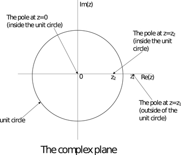
Figure 7. The unit circle in the complex plane showing the poles. The poles z = 0 and z = z2 are inside the unit circle.
Download figure:
Standard image High-resolution image
z = 0 pole of f(z) is obviously inside the unit circle, and it is a pole of order 2. Both the roots z1 and z2 are poles of order 1, but only z2 lies inside the unit circle, as shown in figure 7. It can be checked readily that this is true regardless of whether  or
or  . It's not of importance to consider the case
  , for, this particular case will not have any effect on the final expression for J1. The reason for that is as follows.
  being just one point on the
  -axis is of measure 0. Hence, it will not contribute to the integration w.r.t. the
  variable immediately following the
  integration in the evaluation of J1.
The residues of f(z) are evaluated at z = 0, and z = z2, the only poles inside the unit circle, using the following formulae. z = z2 being a simple pole,  . Next, z = 0 being a pole of order 2,
 ![${Res}(f(z)){| }_{z=0}={\mathrm{lim}}_{z\to 0}\tfrac{d}{{dz}}\left[{z}^{2}f(z)\right]$](https://content.cld.iop.org/journals/2399-6528/5/1/015009/revision3/jpcoabd69aieqn324.gif) . Evaluating the residues and subsequently adding them together, after some algebra, one obtains a rather simple result:
. Evaluating the residues and subsequently adding them together, after some algebra, one obtains a rather simple result:  . [The algebra involves repeated use of the identity z1
z2 = 1, the validity of which can readily be checked from equation (C4)]. Replacing
. [The algebra involves repeated use of the identity z1
z2 = 1, the validity of which can readily be checked from equation (C4)]. Replacing  by − 2iz2 in equation (C3), one obtains the following expression for the contour integral ∮dzf(z).

Using equation (C5) in equation (C1), with z2, as given in equation (C4), one obtains,

There are two  integrals in equation (C6), which is a direct result of the fact that z2, as can be seen from equation (C4), assumes two different expression for the the two regions:
  or
or  . For
. For 
 , and for
  ,
,  . What happens at
  is a moot point here, since, as mentioned before, a single point
  , being of measure 0, does not contribute to the
  -integral in equation (C6).
Our goal is to obtain, analytically, an expression for J1 in terms of small DEM  . We will bypass evaluating the integrals in equation (C6) in closed form, by Taylor-expanding them for small
  . To that end equation (C6) is first written in the following way.

where,


Next  and
and  are Taylor-expanded for small
  . First,
  is expanded around the point
  as follows.
  . We truncate the Taylor expansion up to the
  term, so that, as per equation (C7), the factor
  multiplying
  , will produce terms upto
  . It is our goal to keep the energy expansion up to
  . This is in line with the polaron energy calculations in conventional polar crystals, in which the
  term gives the mass correction of the electron due to polaron formation.
  can be calculated from equation (C8a
) using the second fundamental theorem of integral calculus, as per which,
can be calculated from equation (C8a
) using the second fundamental theorem of integral calculus, as per which,  is simply the integrand of equation (C8a
) with
is simply the integrand of equation (C8a
) with  being replaced by the variable
  . So,
. So,

Calculating  , etc from equation (C9) is straightforward. The derivatives of ψ are calculated up to the order 4, and are evaluated at
  , to give,
  and
and  . Using these in the above-mentioned Taylor-expansion of
  about
about  , one obtains

In an exactly analogous way,  can be Taylor-expanded using the integral given by equation (C8b
). We simply mention the result in the following.
can be Taylor-expanded using the integral given by equation (C8b
). We simply mention the result in the following.

 has been expanded upto
  , since there is already an
  term multiplied to it in equation (C7), and our goal is to keep the J1 in equation (C7) upto
  . Using equation (C10) and equation (C11) in equation (C7) one obtains

The expression for J1 in equation (C12) is the same as that of J1 in equation (B6) up to  .
.
C.2. Evaluation of J2
In this appendix we will show that the leading contribution of J2, given by equation (B5b
), is  . Expressing
  and
and  in terms of z, J2 can be written in terms of the contour integral of the complex variable z ≡ ei
ϕ
as follows
in terms of z, J2 can be written in terms of the contour integral of the complex variable z ≡ ei
ϕ
as follows

where

The function h(z) in equation (C14) has a pole of order 3 at z = 0. There are two other poles of h(z), of order 1, viz., z1 and z2, which are the same ones as given by equation (C4). Just like before, of all the three poles, only two, viz., 0 and z2 are inside the unit circle, as shown in figure 7. Hence the residues of h(z) have to be evaluated only at z = 0, and z = z2 in order to obtain ∮dzh(z). z2 being a simple pole, the residue of h(z) will be given by  . z = 0, being a pole of order 3,
 ![${Res}(f(z)){| }_{z=0}={\mathrm{lim}}_{z\to 0}\tfrac{1}{2}\tfrac{{d}^{2}}{{{dz}}^{2}}\left[{z}^{3}f(z)\right]$](https://content.cld.iop.org/journals/2399-6528/5/1/015009/revision3/jpcoabd69aieqn371.gif) . Evaluating and then adding these residues together, after some algebra involving the repeated use of the identity z1
z2 = 1, one obtains a rather simple result:
. Evaluating and then adding these residues together, after some algebra involving the repeated use of the identity z1
z2 = 1, one obtains a rather simple result:  . This, along with equation (C3), gives the following expression for the contour integral.

Using equation (C15) in equation (C13), after having replaced z2 as given in equation (C4), one obtains the following expression for J2

Equation (C16) needs to be expanded for small  , as was done in case of J1. To that end, equation (C16) is written in the following form first.

where the functions  , and
, and  are given by


We will next apply the Taylor expansion method to the integrals given by equation (C18). Since, we are interested in terms up to  in equation (C17), we need to expand
  upto
upto  and
and  upto
upto  . As for
  given by equation (C18a
), using the second fundamental theorem of integral calculus, one can write
given by equation (C18a
), using the second fundamental theorem of integral calculus, one can write  . From this expression it is possible to compute derivatives of
  of orders up to infinity. Hence it is a matter of straightforward calculation to show that
  . Also,
  , as is obvious from equation (C18a
). Hence Taylor expanding
, as is obvious from equation (C18a
). Hence Taylor expanding  up to
up to  ,
,  . Hence there is no contribution of
  to J2 up to
  .
.
As for  ,
,  , as can be seen from the definition of β as given by equation (C18b
). For small
, as can be seen from the definition of β as given by equation (C18b
). For small  , the first leading order term in
  is
is  . Hence
  term in equation (C17) does not have any contribution up to
  . Hence neither
  , nor
, nor  contribute to J2 in equation (C17) up to the order of our interest. Hence following equation (C17), J2 assumes the following form.


C.3. Evaluation of J3
Finally, we will show that the leading order term of J3, as given in equation (B5c
), is  . To that end we will first carry out the
  integration by our standard technique of replacing the
  integration by the contour integration w.r.t
  . Replacing
  by
by  and
and  by
by  in the expression for J3, and changing
  to
to  , J3 assumes the following form

where

The function t(z) has a pole of order 4 at z = 0. There are two other poles of order 1: z1 and z2 of t(z), which are the same ones as given by equation (C4). As was the case for J1 and J2, of all the three poles only two, viz., 0 and z2 are inside the unit circle, as shown in figure 7. z2 being a simple pole, the residue of t(z) will be given by  . z = 0, being a pole of order 4,
 ![${Res}(t(z)){| }_{z=0}={\mathrm{lim}}_{z\to 0}\tfrac{1}{3!}\tfrac{{d}^{2}}{{{dz}}^{2}}\left[{z}^{3}t(z)\right]$](https://content.cld.iop.org/journals/2399-6528/5/1/015009/revision3/jpcoabd69aieqn412.gif) . Evaluating all of these residues and adding them together, after some algebra involving the use of the identity z1
z2 = 1, one obtains:
. Evaluating all of these residues and adding them together, after some algebra involving the use of the identity z1
z2 = 1, one obtains:  . Using this in the residue theorem of equation (C3), the following is derived.

Using equation (C22) in equation (C20), after having replaced z2 as given in equation (C4), one obtains the following expression for J3

J3 can be expanded for small  , in exactly the same way as was done for J1 and J2. It can be shown that the first integral in equation (C23) does not have any contribution upto
  . The first non-zero term of the second integral in equation (C23) can be shown to be of
  , which will be sole contributor to J3 upto
  . Evaluating that term, one obtains the following expression for J3.

J3 in equation (C24) is  as mentioned in equation (B6). In figure 8, how various integrals contribute to ΔEBLG
at different orders of
as mentioned in equation (B6). In figure 8, how various integrals contribute to ΔEBLG
at different orders of  is explained schematically.

Figure 8. Block diagram showing contributions of various integrals to ΔEBLG .
Download figure:
Standard image High-resolution image
Appendix D.: Evaluation of the relaxation rate for BL graphene electrons
Having written  as
as  ,
,  integral in equation (15) will be carried out first [7]. The argument of the δ function in equation (15) is written as

Next the following identity involving a delta-function is used in equation (15).  , where qi
's are the zeros of the function
, where qi
's are the zeros of the function  . Thus equation (15) assumes the following form.

The qi
's appearing in equation (D2) are  , as obtained by solving the equation
  , with
  given by equation (D1). From the expressions of qi
's above, it is clear that
given by equation (D1). From the expressions of qi
's above, it is clear that  should be greater than
  for the qi
's to be real and positive. That sets an upper limit to the range of the variable
for the qi
's to be real and positive. That sets an upper limit to the range of the variable  in the integration w.r.t
  : instead of varying from 0 to 2π,
  will vary from 0 to
  . This is accompanied with a multiplication of the integrand in equation (D2) by a factor of 2, owing to the fact that
  crosses the constant value
  twice, when it does, as
  varies from 0 to 2π. Using the above-mentioned qi
's, as well as properties of δ function, the
varies from 0 to 2π. Using the above-mentioned qi
's, as well as properties of δ function, the  integral in equation (D2) can be carried out to yield the following expression for the relaxation rate
  for BL graphene.
where

Appendix E.: Evaluation of the relaxation rate for SL graphene electrons
In equation (18) the argument of the δ function is written as

Using  , where qi
's are the zeros of
, where qi
's are the zeros of  , one can write equation (18) as follows.

The qi
's appearing in equation (E2) are  , as obtained by solving the equation
  , where
  is given by equation (E1). From the above-mentioned expressions of qi
's, it is clear that
is given by equation (E1). From the above-mentioned expressions of qi
's, it is clear that  should be greater than
  , for the qi
's to be real and positive. That sets an upper limit to the range of the variable
, for the qi
's to be real and positive. That sets an upper limit to the range of the variable  in the integration w.r.t
  : instead of varying from 0 to 2π,
  will vary from 0 to
  . This is accompanied with a multiplication of the integrand in equation (E2) by a factor of 2, owing to the fact that
  crosses the constant value
  twice, when it does, as
  varies from 0 to 2π. Using the above-mentioned expressions for qi
's, as well as properties of δ function, the
varies from 0 to 2π. Using the above-mentioned expressions for qi
's, as well as properties of δ function, the  integral in equation (E2) can be carried out to yield the following expression for the relaxation rate
  for SL graphene.
where

Appendix F.: Evaluation of the relaxation rate for Semi-Dirac electrons
In equation (23) we will first integrate out the  variable. To that end we will treat the argument R of the δ function, given by equation (22b
), as a function of the variable
variable. To that end we will treat the argument R of the δ function, given by equation (22b
), as a function of the variable  . Making use of the identity
  , where
  's are the zeros of the the above-mentioned function
  , one can write equation (23) as follows.

The  appearing in equation (F1), which can be found easily by solving for the equation
  , are given by

In equation (F2) '±' corresponds to the two roots, i = 1, 2. Equation (F2) sets limits on the possible values of  , since the expression inside the third bracket on the right side of equation (F2) has to be greater than 0, for
  to have any real solution. Mathematically,
 ![$\left[{\left(\sqrt{\tfrac{1}{4}{{l}_{x}^{{\prime} }}^{4}+{{l}_{y}^{{\prime} }}^{2}}-1\right)}^{2}-\tfrac{1}{4}{({l}_{x}^{{\prime} }-{q}_{x}^{{\prime} })}^{4}\right]\gt 0$](https://content.cld.iop.org/journals/2399-6528/5/1/015009/revision3/jpcoabd69aieqn464.gif) , which restricts the values of
, which restricts the values of  as follows.

Using equation (F2) in equation (F1), as well as using the appropriate limits of  commensurate with the inequality (F3), as the limits of integration in equation (F1), one obtains the following expression for the relaxation rate for semi-Dirac
where ![${L}_{3}\equiv {\left[{\left(\sqrt{\tfrac{1}{4}{{l}_{x}^{{\prime} }}^{4}+{{l}_{y}^{{\prime} }}^{2}}-1\right)}^{2}-\tfrac{1}{4}{({l}_{x}^{{\prime} }-{q}_{x}^{{\prime} })}^{4}\right]}^{\tfrac{1}{2}}$](https://content.cld.iop.org/journals/2399-6528/5/1/015009/revision3/jpcoabd69aieqn467.gif) , and
, and