

Abstract
Understanding the climatic drivers of present-day agricultural yields is critical for prioritizing adaptation strategies to climate change. However, unpacking the contribution of different environmental stressors remains elusive in large-scale observational settings in part because of the lack of an extensive long-term network of soil moisture measurements and the common seasonal concurrence of droughts and heat waves. In this study, we link state-of-the-art land surface model data and fine-scale weather information with a long panel of county-level yields for six major US crops (1981–2017) to unpack their historical and future climatic drivers. To this end, we develop a statistical approach that flexibly characterizes the distinct intra-seasonal yield sensitivities to high-frequency fluctuations of soil moisture and temperature. In contrast with previous statistical evidence, we directly elicit an important role of water stress in explaining historical yields. However, our models project the direct effect of temperature—which we interpret as heat stress—remains the primary climatic driver of future yields under climate change.
Export citation and abstract BibTeX RIS
Introduction
Agriculture plays a fundamental role in the global fight against poverty, conflict, and social instability [1, 2]. In addition, it is a vital part of the rural economy and an essential component of national security and foreign policy [3–5]. As climate changes, nations face the mounting challenge of feeding nearly nine billion people by the middle of the century [6, 7]. Yet, over 80% of cultivated lands are not equipped for irrigation in the United States (US) as well as globally, leaving them vulnerable to the shocks of droughts and heat waves [8]. Identifying future threats to rain-fed agriculture is therefore paramount to scientific and policy communities alike and doing so necessitates techniques for characterizing the distinct climatic stressors that affect present-day crop yields [9, 10].
A growing empirical literature has consistently documented a robust negative relationship between high summer temperatures and rain-fed crop yields and the resulting large damages associated with a warming climate [11–16]. However, the biophysical interpretation of these results is not clearly established, such as the extent to which temperature-driven damages reflects changes in heat or water stress. In fact, much less is known about the large-scale statistical relationship between rain-fed crop yields and water availability. Unlike temperature, characterizing the effects of water on crop yields is less obvious in a statistical framework. For instance, variables that are commonly used to represent the supply of water, such as monthly or total growing-season precipitation, explain surprisingly little variation in historical and projected yields (e.g. [11]).
In this study we link detailed soil moisture and temperature data with a large panel of county-level agricultural data (1981–2017) to unpack the historical and future climatic drivers of yields for six major US crops: maize, soybeans, winter wheat, spring wheat, cotton and sorghum (figures S1–S7 is available online at stacks.iop.org/ERL/14/064003/mmedia). These crops represent about 90% of the national farmland devoted to field crops and constitute a major portion of the global supply of maize (37%), soybeans (34%), sorghum (17%), cotton (14%) and wheat (9%). Our analysis focuses on non-irrigated US counties, which encompass most of the national harvested area in maize (86%), soybeans (93%), winter wheat (96%), spring wheat (88%), cotton (55%) and sorghum (96%).
Unpacking the climatic stressors of crop yields requires improving the statistical characterization of the yield-water relationship. A natural first step is to adopt more direct measures of soil water content. The evolution of soil moisture over time reflects the changing balance between water inflows (e.g. rainfall, irrigation) and outflows (e.g. runoff, percolation, evapotranspiration), and thus accounts for the effect of complex meteorological and hydrological processes that are difficult to account for explicitly in a statistical crop yield model (e.g. rainfall variability and intensity, evaporative demand of warmer temperatures or dry atmospheric conditions). Unfortunately, unlike meteorological data, there is no extensive network of soil moisture monitoring stations. We thus rely on state-of-the-art land surface model (LSM) data from the North American Land Data Assimilation System (NLDAS), a major collaboration between NOAA, NASA, Princeton University and the University of Washington. The NLDAS provides hourly estimates of soil moisture content for different soil layers based on four different LSMs at a 1/8th-degree spatial resolution (∼14 km). These LSM data have been validated against observations [17] and constitute, to our knowledge, the best long-term estimates of soil moisture content for North America and thus an improvement in the representation of water availability for crops over large areas relative to precipitation or simple measures of water balance.
Improving the characterization of the yield-water relationship also requires recognizing the critical role of the intra-seasonal timing of environmental stress in crop yield determination [18, 19]. To this end, we harness the temporal granularity of soil moisture and air temperature data to estimate a flexible model that can detect variations in the distinct effects of these climatic drivers of crop yields throughout the growing season. Improving how we represent the relationship between the timing of soil water content and crop yields is a critical first step before more sophisticated statistical models and projections with improved bio-physical grounding can be developed.
Our main analysis is based on a statistical panel model that jointly estimates the distinct within-season effects of soil moisture and temperature fluctuations on crop yields (see Materials and Methods). Importantly, our approach harnesses the year-to-year deviations at each location in the data to estimate the yield contribution of environmental conditions throughout the growing season. This avoids confounding average environmental conditions with fixed unobservable drivers of yield. This also means that our estimates only account for short-run adaptations to environmental change that farmers can undertake as the growing season unfolds. We project future yield losses by linking our yield model estimates with climate projections from general circulation models (GCM) of the climate model intercomparison project phase 5 (CMIP5) forced with various representative concentration pathways (RCPs). RCPs are scenarios with varying levels of climatic forcing. The Supplementary Materials provide additional results exploring the robustness of our results.
Results
Yield sensitivities to intra-seasonal soil moisture fluctuations
We find crop yields exhibit sensitivities to soil moisture that vary considerably throughout the growing season and are particularly pronounced around mid-season. We report estimates for the effect of soil moisture on crop yields throughout the growing season in figure 1(A). The figure has six sub-panels, each representing the marginal effect of soil moisture (vertical axis) at different stages of the growing season for each crop (horizontal axis). To facilitate comparisons, we normalize the length of the growing season to 100%, which means that the estimated response surface (colored surface) depicts the yield percent contribution of spending 1% of the growing season at a particular level of moisture. We also depict the sample's historical distribution of soil moisture (vertical axis on the right) over the growing season. The response surface thus indicates how a particular weekly sequence of moisture exposures over the season, or moisture path, cumulatively contributes to yield at the end of the season. Red areas indicate moisture levels that are detrimental to yields at certain periods of the growing season, whereas blue areas indicate moisture levels that contribute positively to yield. For clarity, figure S8 shows 'cross-sections' of the response surface and its confidence band evaluated at different levels of season progress.
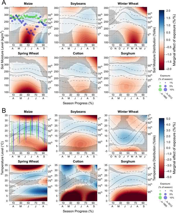
Figure 1. Intra-seasonal effects of soil moisture (A) and temperature (B) exposures on crop yields. Each sub-panel presents a response surface illustrating how the marginal effects of moisture (A) and temperature (B) on crop yield varies over the growing season. The x-axis represents the timing in the growing season or season progress (%) and the y-axis represents either soil moisture level (A) or temperature (B). The response surface represents how spending a 1% fraction of the growing season at a specific level of moisture or temperature affects crop yield. Dashed lines in each panel represent percentiles of the historical distribution of soil moisture or temperature throughout the growing season. The colored circles in the maize sub-panels (top left in panels (A) and (B)) correspond to levels of exposure in 1985 (green) and 2012 (blue), in McLean County, Illinois, which the largest maize-producing county in the United States. The size of those circles represent the level of exposure (in % of the season). The exposures for a 'good' year (1985 with a 31% increase in yield) and a 'bad' year (2012 with a 40% decrease in yield) in that county illustrate the critical role of moisture and temperature changes around the various portions of the growing season. The statistical uncertainty of the model is captured with 1000 bootstraps whereby observations are blocked by year. The shaded regions indicate marginal effects that are not statistically different from zero. This uncertainty is also shown for select levels of season progress in figures S8, 9. Note that the scale on the x and y axes vary depending on the crop and the panel.
Download figure:
Standard image High-resolution imageRelatively low levels of soil moisture around the middle portion of the growing season are particularly damaging to yields for all crops. In the case of maize, traversing the 20% portion of the growing season between 40% and 60% of season progress at a soil moisture level of 150 kg m−3, where the marginal effect of moisture exposure is approximately −1.4%, suggests a 28% yield reduction (−1.4 × 20) from the county average. This is consistent with the notion that crop yields are particularly sensitive to water stress during specific stages of crop development [18, 19]. For instance, water stress can irreversibly affect the viability of flowering and fertilization and reduce the rate of biomass accumulation during grain-filling [20].
Slightly dry conditions appear beneficial toward the very end of the season for crops like maize, spring wheat and cotton. This may reflect the fact that dry conditions are favorable for harvest. On the other hand, wet soils are generally beneficial around the middle of the season. In contrast, very wet conditions appear detrimental, either towards the beginning or the end of the season depending on the crop. This is consistent with the idea that excessive moisture is detrimental for plant field establishment and is undesirable at harvest, such as for cotton, for which excessive rainfall at harvest can lead to boll shedding thus reducing yield.
We illustrate the intra-seasonal effects of soil moisture with an example. We overlaid the weekly moisture exposures of two different years, 1985 and 2012 (in green and blue, respectively), in the largest maize-producing county in the sample (McLean County, IL) on top of the response surface for maize in figure 1(A). In both years, early-season moisture levels were around median historical sample conditions. However, the 1985 moisture path remained consistently above median levels, leading to above-average yield in that county (+29%). In contrast, precipitation deficits and high temperatures in the late Spring of 2012 resulted in a rapid drying of soils that coincided with the sensitive middle part of the growing season, leading to below-average yield in this county (−41%). Note that moisture levels recovered later in the season due to late summer precipitation but large damages had already accrued.
Yield sensitivities to intra-seasonal temperature fluctuations
We also find crop yields exhibit sensitivities to temperature that vary throughout the growing season with relatively hot conditions (>30 °C) appearing detrimental during warm parts of the growing season. We report estimates for the marginal effect of temperature (vertical axis) on crop yields throughout the growing season (horizontal axis) in figure 1(B). The interpretation of the temperature response surface is analogous to that of soil moisture. We also represent the temperature response function and its confidence band evaluated at different levels of season progress in figure S9. Exposure to relatively high temperature (>30 °C) over warmer parts of the growing season appear particularly damaging to yields for most crops. For instance, in the case of maize, spending 1% of season exposure (∼44 h) in the middle of the growing season (June and July) at 35 °C suggests a 5.9% yield reduction from the county average. For most crops, the damaging effects of higher temperature are reflected throughout much of the season. For cotton, the damaging effects of high temperatures appear concentrated in the second half of the growing season (July and August) when cotton is setting bolls (see figure S3). For winter wheat, which has a growing season spanning two calendar years, the detrimental effects of high temperature are perceptible in the Spring (March). Note that sorghum appears about half as sensitive to high temperature than maize.
Exposure to relatively cool temperatures appear somewhat detrimental to most crops, particularly for sorghum. Interestingly, exposure to temperature around 5 °C–10 °C for winter wheat seem beneficial during the winter months (December and February), which could reflect the effect of vernalization, whereby exposure to cool winter conditions help induce flowering in the spring.
The effects of temperature on crop yields exhibit less intra-seasonal variation than soil moisture effects. For instance, dry or wet soil moisture conditions appear particularly detrimental around relatively short portions of the growing season for all crops, whereas high or low temperatures appear detrimental largely throughout the growing season for most crops. That is, intra-seasonal effects for temperature appear more temporally additive than for soil moisture.
We also overlay the monthly temperature exposures for 1985 and 2012 in McLean County, IL on top of the temperature response surface for maize in figure 1(B). In both years, early-season temperature distributions (April) appeared similar, but exposure to temperatures above 30 °C in the summer (e.g. July) was more pronounced in 2012.
Eliciting greater role of water in explaining historical yields
We examine six different models to assess how accounting for intra-seasonal environmental effects and soil moisture content improves statistical fit. Figure 2 shows the reduction in root mean square error (RMSE) of out-of-sample predictions of each model relative to a baseline model that excludes environmental variables. This captures the share of the historical yield variation around the trend of each crop explained by the statistical model. RMSE is computed following a ten-fold cross-validation in which years of data are sampled, which is a common approach for model and variable selection [21].

Figure 2. Reduction in root mean square error (RMSE) for alternative models. The reduction is computed relative to a model with a state-level quadratic time trend and without weather variables and based on a ten-fold cross-validation (see Methods). The models include a (i) 'season-long precipitation' model including linear and quadratic terms for total growing-season precipitation, (ii) an 'intra-seasonal moisture' model including our proposed moisture variable, (iii) a 'season-long temperature' model including nonlinear effects of temperature which are additive over the growing season, (iv) an 'intra-seasonal temperature' model including our proposed temperature variable, (v) a traditional 'season-long temperature and precipitation' model that combines the season-long precipitation and temperature models, and (vi) the proposed 'intra-seasonal moisture and temperature' model that combines the intra-seasonal moisture and temperature models.
Download figure:
Standard image High-resolution imageAllowing for intra-seasonal moisture effects (model ii) improves prediction accuracy by between 84% and 424% relative to a model based on season-long precipitation alone (model i), which is a standard in the literature. Similarly, accounting for intra-seasonal temperature effects (model iv) improves prediction accuracy by between 7% and 63% relative to a model that assumes additive season-long temperature effects (model iii). The gains from accounting for intra-seasonal temperature effects (model iv versus iii) appear smaller than from accounting for intra-seasonal moisture (model ii versus i), suggesting that timing considerations are particularly important for capturing the role of water stress.
Comparing the full models, our proposed model allowing for both intra-seasonal soil moisture and temperature effects (model vi) outperforms a traditional model based on season-long temperature and precipitation (model v) by between 15% and 115%. Note that predictions improve, although not additively, when intra-seasonal measures of soil moisture and temperature are combined, suggesting that these variables partly explain a common source of variation in crop yields. Indeed, droughts and heat waves often coincide raising the potential concern of multicollinearity of soil moisture and temperature variables. Multicollinearity is problematic because it renders parameter estimation less precise, deteriorating a model's ability to predict out of sample. However, model vi improves prediction accuracy relative to all other models we consider suggesting that moisture and temperature variables confer distinct predictive power.
Vulnerabilities to soil moisture and temperature change
To explore the vulnerabilities of crop yields to changes in moisture and temperature, we consider the effect of idealized climate change scenarios applied to our model. Figure 3 reflects the yield impact for the full sample from uniform changes in soil moisture and temperature during a critical month of the season for each crop (see Materials and Methods). These uniform scenarios cover a much wider range of climate stresses than simulated by the CMIP5 models alone.
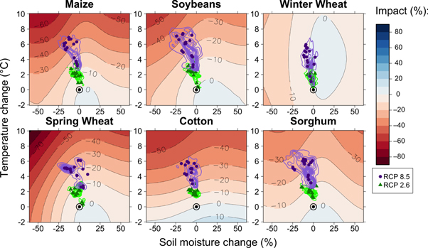
Figure 3. Crop yield projections from uniform changes during a critical month of the growing season. The identification of the critical month for maize (July), soybeans (August), winter wheat (March), spring wheat (June), cotton (July) and sorghum (July) is discussed in Methods. Yield projections are area-weighted to represent current rain-fed growing regions analyzed in our sample. The circled dot represents the current climate. Each circle or triangle represents an individual GCM projection (CMIP5) during the critical month for 2050–2100. The purple and green contour lines represent the joint-distribution of county-level temperature and moisture projections for all GCMs based on current growing regions.
Download figure:
Standard image High-resolution imageYield impacts from changes in environmental stressors tend to be asymmetric for most crops with more pronounced yield declines resulting from dryer and hotter conditions than yield gains from wetter soils and cooler conditions relative to historical baseline conditions (table S1). For instance, a 20% drop in moisture in July decreases maize yields by about 12% whereas an equivalent moisture increase barely affects yield. Similarly, a 2 °C increase in temperature in July decreases maize yields by 6.8% whereas an equivalent drop in temperature raises yield by just 2.8%.
Importantly, the vulnerability to moisture change cannot not be identified explicitly with a traditional model based on growing-season precipitation (see Materials and Methods; figure S11). A similar analysis for a traditional model indicates that even the most extreme changes in precipitation (e.g. by a 100% reduction) have a limited bearing on the overall impacts (figure S11), and this is regardless of whether meteorological variables are confined to a critical month (figure S12).
Major role of temperature in explaining future yields
To illustrate how modeled climate change projections are situated within this space of idealized projections, we overlay CMIP5 projections for the critical month of each crop in figure 3 for the mildest (RCP 2.6, in green) and most severe climate scenarios (RCP 8.5, in purple). Each circle represents a sample-wide climate projection under a particular GCM. CMIP5 climate change projections indicate a clear and pronounced warming and a more tenuous drying pattern. Although crop yields are found to be fairly sensitive to moisture changes historically, our models suggest temperature change appears to emerge as the primary climatic driver of future yields under CMIP5 projections. Figure 3 also forewarns of considerably larger yield damages if drying slightly exceeds current CMIP5 projections during key parts of the year.
Projected climate change impacts
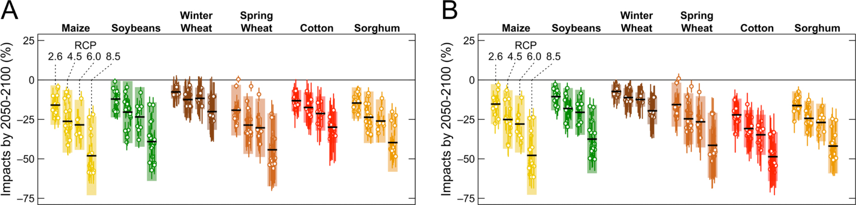
Overall, we find that under current production systems and practices, our models indicate aggregate crop yields could decrease during the end of the century (2050–2100) by 8%–19% under the mildest scenario (RCP 2.6), and by 20%–48% under the most severe scenario (RCP 8.5). Our yield projections are relative to a baseline without climate change and do not reflect secular trends in crop yields resulting from technological progress that may well continue. Yield projections during the end (2050–2100) and the middle of the century (2025–2075) are depicted in figure 4(A) and figure S13(A), respectively, and summarized in table S2.

Figure 4. Climate change impact projections on United States crop yields. Each dot represents a particular GCM in CMIP5 for the end of the century (2050–2100). Vertical lines around each dot represents the 95% confidence interval based on a block bootstrap procedure whereby years of the data are sampled with replacement. The horizontal solid black line and the colored bands correspond to the mean and ± two standard deviation of each ensemble, respectively. Climate change scenarios are increasingly severe from RCP 2.6–8.5 (see Materials and Methods). (A) Proposed model accounting for intra-seasonal effects of soil moisture and temperature. (B) Traditional model with constant intra-seasonal effects of precipitation and temperature.
Download figure:
Standard image High-resolution imageFigure 4(A) shows projections for all six crops under four RCPs scenarios where each circle represents an average sample-wide yield projection under a particular CMIP5 model. The vertical tick marks represent 95% confidence intervals capturing the statistical uncertainty in the regression model and not climate-projection uncertainty. The confidence intervals are computed based on a year block-bootstrap which accounts for contemporaneous spatial dependence.
The wide colored bands represent ± two standard deviations of individual CMIP5 yield projections for the full sample around the ensemble mean, which is represented by a horizontal black line. These bands capture the uncertainty in climate projections and not the uncertainty associated with the statistical model. In general, yield projections exhibit climatic uncertainties that exceed their statistical uncertainty. The climatic uncertainty stems from the variability of projected changes in climatic factors across different GCMs, whereas the statistical uncertainty stems from the estimation of the historical crop-environment relationship.
Similar sample-wide climate impacts with a traditional model
We contrast our climate change impact projections to those of a traditional model based on total growing-season precipitation and temperature exposure, similar to the model developed in [11]. This model assumes weather effects are additive over the growing season and is based on total growing-season precipitation and temperature exposure. Yield projections for the traditional model during the end (2050–2100) and the middle of the century (2025–2075) are depicted in figure 4(B) and figure S13(B), respectively. Results for both periods are summarized in table S3.
Overall, we find our projected impacts for the full sample (figure 4(A)) remain comparable to the traditional model (figure 4(B)), except for cotton. For each GCM, we assess whether the projected impacts differ statistically between both models (table S4). We find that impacts are virtually indistinguishable at 5% and 10% critical levels for a majority if not all GCMs for all crops, except cotton, for which multiple projections appear to differ. In the case of cotton, our proposed model points to climate change damages that are, on average, about 40% smaller across all GCMs, scenarios and projection periods.
Decomposing climatic drivers of future yields
To understand the climatic factors driving crop yield impacts in our model relative to previous approaches, we decompose the contribution of different types of variables to overall climate change impacts. Figure 5 shows this decomposition for all crops and during the end of the century for the proposed model (A) and the aforementioned traditional model (B). We show the decomposition for the middle of the century in figure S14.

Figure 5. Decomposition of climate change impact projections on United States crop yields. Decomposition into water-related variables (precipitation or moisture) and temperature for the end of the century (2050–2010). Each colored bar represents the CMIP5 ensemble mean contribution to yield impacts for each type of variable. Each dot represents the contribution of the variable to yield impact for a particular GCM. (A) Proposed model accounting for intra-seasonal effects of soil moisture and temperature. (B) Traditional model with constant intra-seasonal effects of precipitation and temperature.
Download figure:
Standard image High-resolution image
Impacts are overwhelmingly driven by changes in temperature in the traditional model (figure 5(B)) whereas they are driven by a combination of both moisture and temperature effects in our approach (figure 5(A)). The contrast between these two models is even more pronounced for the middle of the century because of a smaller role of temperature in driving overall impacts (figure S14). Results also indicate that the greater contribution of soil moisture to overall impact projections in our model are linked to a smaller impact of temperature change. This suggests that the new soil moisture variables capture a sizable portion of the effect of water stress that had been embodied in the temperature effects in previous traditional models.
Greater moisture-driven heterogeneity of local climate change impacts
Plotting county-level climate change impact projections for the proposed model against those for the traditional model (figures S15, S16) reveals important discrepancies in local impacts, particularly for winter wheat, spring wheat and cotton. To verify the source of such discrepancies, we plot, for each model, the yield contribution of climatic drivers in every county for all RCP scenarios. The traditional model suggests that the contribution of precipitation change to total yield impact for virtually every county in the sample is almost negligible (figures S17, S18). In contrast, the proposed model suggests that the contribution of soil moisture change to total yield impact varies considerably across counties in the sample (figures S19, S20). Thus, modest differences in sample-wide impact projections between the proposed and traditional approaches conceal considerable local county-level discrepancies.
Discussion
Methods for unpacking climatic drivers
Assessing the impact of environmental factors on crop yields can be done through biophysical or statistical approaches. Biophysical approaches model the underlying physiology of crop yield formation as affected by sub-daily weather conditions and pre-determined management decisions. These models have been better suited for unpacking the environmental factors affecting yields, such as heat or water stress [22]. However, these models are not directly grounded in observational data so they do not necessarily reflect yield responses under real-world conditions farmers face. In addition, predictions based these models can diverge considerably under extreme climate scenarios [23].
Statistical crop yield models, on the other hand, are based on regression analysis and link observed yields with relatively simple weather predictors. These models are relatively simple to implement and their empirical grounding means they implicitly reflect real farmer behavior. However, the effects of individual weather variables in these models do not have clear biophysical interpretations, hindering the attribution of yield damages to either heat or water stress.
Interpreting temperature effects
A recurrent finding in statistical studies is the major detrimental role of high temperature (and the relatively minor role of precipitation) in explaining historical and future rain-fed crop yields (e.g. 10–15). Recent biophysical evidence suggests that high temperature may be detrimental to maize yields because it increases evaporative demand, causing water stress [24]. This implies that statistical model projections, which have been mostly temperature-driven, may indirectly reflect the effect of rising water stress on future rain-fed crop yields under climate change.
On the other hand, climatological evidence indicates that high temperature is often caused by large-scale precipitation deficits [25]. Thus, high temperature may simply appear detrimental to rain-fed crop yields in statistical settings because it is simply correlated with water stress. If correct, this may be problematic for projecting future crop yields, because while high temperatures and moisture deficits have been correlated historically, their coupling may vary under a different climate [26]. This could render temperature-driven statistical model projections less reliable [27].
A key challenge is determining to what extent do temperature effects in statistical studies capture heat or water stress. The distinction is important because these two types of stresses involve different physiological mechanisms [20] and understanding their relative role is critical for prioritizing policy initiatives and research efforts to make rain-fed agricultural systems more resilient [7].
Towards improved interpretations of statistical models
A good indication of scientific progress in the climate change impacts literature is the growing consensus in the conclusions of studies based on different methodological approaches. It is encouraging that a rising number of comparative studies find that statistical models point to similar yield projections than their biophysical counterparts, at least for moderate climate change scenarios [28–31].
However, the biophysical underpinnings of statistical crop models remain deficient. For instance, the statistical literature has yet to establish whether temperature effects are primarily reflecting soil moisture deficits or whether they may also reflect heat stress. This is important because it enhances our ability to craft proactive adaptation strategies to a changing climate, such as crop breeding for heat or drought tolerance.
In this study we seek to improve our ability to unpack the distinct climatic drivers of future rain-fed crop yields by refining the representation of water-related and time-varying stresses in large-scale statistical models. For this purpose, we rely on detailed measures of soil moisture content from state-of-the-art LSM data. Such soil moisture variables are standard in earth and atmospheric science and are available as outputs of GCMs in CMIP5 but have received little attention in the climate impacts community.
A striking finding of our study is how robust the intra-seasonal differences in crop yield sensitivity to environmental conditions are, particularly for soil moisture. We detect such time-varying effects in all crops which is consistent with conventional wisdom in agronomy that water and heat stress during certain crop stages are particularly detrimental to crop yields [18, 19]. Our approach facilitates the representation of varying intra-seasonal sensitivity that only a few past studies have addressed although in more basic fashion [32–35]. We are thus able to expose vulnerabilities to water stress in rain-fed agriculture that remain obscured in previous large-scale statistical studies, highlighting the fundamental role of precipitation change and variability in climate change modeling and impact analysis. This framework expands the scope of potential insights and types of adaptation that may be explored with statistical methods.
Limitations
Our study presents caveats that bear mentioning. Although we account for variations in intra-seasonal effects of both soil moisture and temperature, we do not model their interactions. This could exacerbate our projected damages. Incorporating interactions increases model complexity exponentially, rendering our model intractable. Future research could explore such linkages, perhaps by extending our approach to a 3D spline allowing parsimonious interactions. Our main impact projections hold growing regions, growing seasons, crop cultivars and sensitivities to environmental conditions at their observed historical levels. These are critical margins of adaptation to climate change that extend beyond the scope of this study. Our projections should therefore be interpreted as plausible upper bounds on climate change damages on US crop yields if all else were to remain the same under the current production system. Finally, our projections do not explicitly account for increases in atmospheric CO2 [36].
Broader implications
It is somewhat reassuring that our sample-wide impact estimates provide comparable overall outlooks than previous statistical approaches based on growing-season and precipitation variables. However, there are noticeable differences for certain crops (e.g. cotton), particularly at the local level. These differences are driven by the variability of local soil moisture projections stemming from CMIP5 projections. While temperature projections point to an overall warming, soil moisture projections are mixed and vary by region and by GCM. Because our modeling approach incorporates this variability, it is naturally translated in our yield projections. This is important because there is more uncertainty regarding projections of the water balance than in changes in temperature, and this uncertainty should be better understood by local and regional planners.
Importantly, our proposed approach points to a different partition of climatic drivers in driving overall climate impacts than previous approaches. Our approach directly elicits a greater role of water-related stress in governing both historical and future yields. However, the direct role of temperature—which we interpret as heat stress in our framework—still remains the primary climatic driver of US rain-fed crop yields under climate change. That being said, rapid advances in land surface modeling will likely further improve the attribution of impacts to distinct climatic stressors. Thus, future studies may improve the partition of climatic drivers of future yield distributions. Our findings are supportive of efforts targeted at enhancing heat tolerance but also drought resistance.
The development on new agricultural technologies that enhance resilient to a changing climate seem particularly urgent. For instance [37, 38], find that agricultural production has become, particularly in the US Midwest, more sensitive to climatic variations over time. This underscores the pressing need for more directed efforts in agricultural innovation given the long lags between the time of R and D investments and their returns [39] and the rapid projected pace of climate change.
The methods we develop open promising new research avenues for analyzing cultivated and natural systems with inherently seasonal linkages with water resources. Empirical researchers can now rely on state-of-the-art LSM historical data and soon on improved LSM data in the upcoming CMIP6 to assess critical challenges of the future climate system that have so far remained elusive.
Materials and methods
Data sources
We rely on county-level crop yield data from USDA/NASS (1981–2017) for six major crops in the United States: maize, soybeans, winter wheat, spring wheat, cotton and sorghum. The analysis is based on an unbalanced panel of rain-fed counties (figures S1) but results remain very similar when confined to the balanced data. We represent crop yields over time in figures S2. We define the growing season for every crop as a calendar period that includes the historical timing of planting or emergence as well as maturation or harvest (figures S3). This corresponds to April–September for maize, soybeans, cotton and sorghum, April–August for spring wheat, and October–June for winter wheat. We considered models accounting matching environmental conditions to phenological crop stages and results remain very similar. However, we favored models based on calendar growing seasons to simplify exposition.
We obtain soil moisture data from the LSM in the NLDAS-2 (https://ldas.gsfc.nasa.gov/nldas/) [17]. The NLDAS provides hourly soil moisture for each 1/8th-degree (∼14 km) for various soil depths (available soil depths vary by LSM) across North America since 2, January 1979. The NLDAS LSMs combine hourly information about multiple atmospheric variables with biophysical land characteristics to derive the state of soil water content over time. We rely on soil moisture for the superficial soil layer (0–10 cm) which is the data we find best predicts crop yields (versus 0–100 cm layer) and that is readily available in future climate projections. This restricted our choice to 3 of the 4 available LSM in NLDAS-2 (NOAH, SAC and MOSAIC). We aggregate hourly data to a weekly time scale. This is in line with the time scales chosen for the United States Drought Monitor. Weekly NLDAS grid-level observations are aggregated to the county level based on cropland area falling within each grid. These weights are computed from USDA's 30 m National Cropland Data Layer (CDL) by computing the average cropland pixels falling within each NLDAS grid in 2008–2014. Weekly variation in soil moisture is shown in figure S4.
For weather data we rely on daily and monthly PRISM data for precipitation, maximum, minimum and average temperature from the PRISM Climate Group (http://prism.oregonstate.edu), which is available since 1981. Daily temperatures are processed into temperature exposure bins necessary to estimate nonlinear effects of temperature similar to [11]. We compute the exposure to each 1 °C bin from −15 °C to 50 °C in each PRISM grid by assuming a double sine curve passing through the minimum and maximum temperature of consecutive days. Gridded weather data is aggregated up to the county using cropland weights based on the CDL. figures S5, 6 show the county-level distributions of monthly precipitation and temperature bins. In figures S7 we show the aggregate growing-season distributions of these variables used in the traditional model that assumes additivity.
Regression models
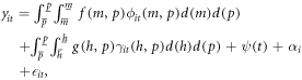
We develop a statistical panel model to estimate the nonlinear and time-varying effects of soil moisture and temperature on crop yield throughout the growing season. The functions  and
and  capture these intra-seasonal effects which represent the marginal yield response to soil moisture level
  or temperature
  at each level of season progress
  The logged yield
  in county
  and year
  can be represented generally as:
where  describes the distribution of soil moisture content and
  the distribution of temperature at each level of the growing season.
  captures a state-level quadratic time trend and
  is a county fixed effect. To estimate this model we approximate the soil moisture
  and temperature
  yield response functions with a bivariate tensor-product or two-dimensional (2D) natural cubic spline. This requires we discretize the
  and
and  into 2D bins. Our 'progress' bins are either weeks for soil moisture or months for temperature. Our 'variable level' bins are equally-spaced for soil moisture (50 bins from 0 to 500 kg m−3) and temperature (66 bins from −15 °C to 50 °C). The resulting dataset reflects the time spent in each 2D bin. To facilitate comparison across crops, we normalize the growing season length to percentages. Prior to the regression analysis, soil moisture bins are aggregated below 100 and above 350 kg m−3 and temperature bins are aggregated below 0 °C and above 35 °C. This avoids relying on bins with little exposure, which leads to noisy estimates for extreme bins.
The regression model is estimated based on a transformed dataset of the 2D binned data, post-multiplied by a 2D B-spline basis matrix. This is a bi-dimensional generalization of previous work estimating nonlinear effects over a single dimension. The 2D B-spline basis matrix result from the outer product of each pair of columns of the individual one-dimensional B-spline matrices of each variable (progress and moisture/temperature). To choose the degrees of freedom in the progress and level dimensions for the soil moisture and temperature response surfaces we conduct a grid search where we independently vary the flexibility of the model and assess the out-of-sample prediction accuracy (figure S44). To favor relatively parsimonious models, we choose levels of model flexibility for which subsequent increases in degrees of freedom do not improve model fit by more than 5%. The appendix provides additional details. Uncertainty of the statistical crop yield model is captured with a year block bootstrap (R = 1000) which preserves the underlying spatial and contemporaneous dependence in the data.
Throughout the paper we contrast the results of our preferred model with those of a traditional model, closely following [11], that treats temperature exposure and precipitation as additive over the growing season. We show how model flexibility affects prediction accuracy for this model in figure S48.
Climate change impacts
Climate change impacts on crop yields are computed as  where
where  is a vector of estimated environmental coefficients and
  a matrix representing the change in the climatology between the reference and projection period of the reconfigured environmental variables used in the estimation. Sample-wide impacts are obtained by weighting county-level impacts by the historical crop acreage (1981–2017). Details about climate projections are provided in the appendix.
Acknowledgments
We thank R E Just, D Lobell, P Mérel, J Melkonian, S Riha, J Tack and D Wolfe for helpful comments in earlier versions of the manuscript.
Funding:
A O-B was supported by NSF grant 1360424 and the USDA National Institute of Food and Agriculture, Hatch/Multi State project 1011555.
Author contributions:
AO-B conceived the study and led the writing of the manuscript. AO-B and HW conducted the statistical analysis. CMC computed and downscaled ensemble of climate projections. AO-B computed climate change impacts. AO-B and TRA interpreted results and climate projections. All authors assisted in writing the manuscript.
Competing interests:
The authors declare that they have no competing interests.
Data and materials availability:
All data needed to evaluate the conclusions in the paper are present in the paper and/or the Supplementary Materials. Additional data related to this paper may be requested from the authors.