

Abstract
We compare predictions of a simple process-based crop model (Soltani and Sinclair 2012), a simple statistical model (Schlenker and Roberts 2009), and a combination of both models to actual maize yields on a large, representative sample of farmer-managed fields in the Corn Belt region of the United States. After statistical post-model calibration, the process model (Simple Simulation Model, or SSM) predicts actual outcomes slightly better than the statistical model, but the combined model performs significantly better than either model. The SSM, statistical model and combined model all show similar relationships with precipitation, while the SSM better accounts for temporal patterns of precipitation, vapor pressure deficit and solar radiation. The statistical and combined models show a more negative impact associated with extreme heat for which the process model does not account. Due to the extreme heat effect, predicted impacts under uniform climate change scenarios are considerably more severe for the statistical and combined models than for the process-based model.
Export citation and abstract BibTeX RIS
1. Introduction
Two distinct approaches have been used to evaluate how climate change will affect agricultural output. One approach takes data and assumptions about soils, solar radiation, management practices and projected daily rainfall and temperatures, and feeds these through process-based mathematical models of plant growth and seed formation (Muchow et al 1990, Jones et al 2003, Keating et al 2003). Impacts from climate change are drawn from differences in yields simulated using historical and projected future weather (Rosenzweig et al 1994). The second approach uses statistical regression models to link historical yield outcomes to historical weather aggregates and extrapolates from observed associations to make predictions about yields under an altered projected climate (Schlenker and Roberts 2009). The two approaches have different strengths and weaknesses. Our goal here is to compare and combine the two approaches using a large new data set that spans a majority of actual maize fields in the United States. Comparison of each model's predictions with actual outcomes allows us to see the circumstances for which each model makes more accurate predictions, and thereby aid future model refinements. Also, by combining models we can likely make more accurate predictions about the potential impacts of weather or climate change.
A key strength of process-based crop models is that they provide a clear physiological mechanism for linking weather to crop yield outcome, with many of the essential parameters in these models having been established through laboratory experiments. If these models can be externally validated (in a predictive sense7), the models can provide more than just a prediction of impacts, but point to an understanding of deeper physiological constraints, which could aid targeted development of adaptive technologies. A challenge with process models is that they are typically validated using data from experimental field plots, and it is not generally clear how well the models can predict outcomes on farmer-managed fields under a range of weather and climate scenarios. Process models include simplifying aggregate descriptions of processes and this might lead to unknown errors in new, untested environmental circumstances. Perhaps more importantly, the models cannot account for factors like pest problems, weed control, fertilizer applications and other management practices that can depend on farmer behavior.
Statistical models have different strengths and weaknesses. Where some statistical analysis makes use of experimental plot data with randomly assigned treatments and management practices, most of it instead uses observational data from individual farms or regions. An advantage of using observational data is that an account of farmer management behavior is implicit, if not observed. Another advantage is the tremendous volume and breadth of available data. And since the weather anomalies are more-or-less randomly assigned by nature, it can be reasonable to ascribe causal links to some kinds of associations between weather and yield outcomes. A shortcoming of statistical models is that associations, even if defensibly causal, can obscure the underlying physiological mechanism that gives rise to the causal link.
The two approaches roughly align with what economists call structural and reduced form methods in applied economics, or what others call model based and design based approaches (Card 2012), a subject of considerable methodological debate (Freedman 1991, Heckman and Urzua 2010, Deaton 2010, Imbens 2010). In recent years, more scholars have begun to see the value in both approaches (Chetty 2009, Timmins and Schlenker 2009, Heckman 2010). We are not aware of similar methodological discussions in the natural sciences.
By simultaneously considering examples of each approach, using a large data set that randomly samples from a near population of fields and spans a wide range of climates and weather outcomes, we draw on the strengths of each approach and work to better understand their weaknesses. Predictions under climate change are likely to be significantly more accurate if they rely on models that are thoughtfully combined, as we attempt to do here. More constructively, we can characterize the circumstances where process models (model based approaches) and statistical models (reduced form approaches) make systematically different predictions, and thereby pinpoint key areas where further research may be most useful. While there was some early work comparing and combining a process model and regression (Irmak et al 2005), there has been little subsequent work, and nothing about which we are aware that attempts an empirical comparison and combination in the manner we do here, or using as large a number of representatively-sampled, field-level outcomes.
2. Data
Field-level data on planting date and crop outcome were obtained from the US Department of Agriculture. The sampled fields (100 randomly-selected fields per county per year from 1995–2012 in each of 12 states, Iowa, Illinois, Indiana, Kansas, Minnesota, Missouri, North Dakota, Nebraska, Ohio, South Dakota and Wisconsin) were taken from a data set that includes a large majority of crop production in the United States. Approximately 90% of the fields had a latitude/longitude location identifier that was used for matching with weather data. All sampled fields included the planting date and a farmer-reported yield outcome.
We omitted observations: (1) for irrigated fields, the vast majority of which were in the warmer and more arid western states, Kansas and Nebraska; (2) with a missing or invalid latitude/longitude location identifier; (3) with a planting date too early to be plausible (before March); (4) with yield outcomes in the top or bottom quarter of one percent; (5) if yield from the process model (briefly described below) was less than 5 bushels per acre; or (6) growing degree days was less than 600 for the assumed 180 day growing period. Finally, we omitted observations from all counties with fewer than 400 total observation across the 18 years. The final data set includes 1 121 601 observations from 741 counties spanning 12 states in the highly productive Midwestern corn belt.
The sampled fields appear to be highly representative of corn production in the 12 states. We demonstrate representativeness in figure 1, which plots the average yield of the 100 sampled fields in each county/year against county average yields reported by NASS. The strong linear relationship with an intercept near zero and slope near one is evident. There are a number of outliers, indicated by the lighter cloud of points indicating sample averages that lie well below NASS-reported yields. Visual inspection of the data indicates that these observations are county-years for which a large number of observations were dropped in the cleaning process described above, mostly due to irrigation. Thus, these outliers can be explained by a combination of larger sample error plus the fact that NASS county averages include irrigated fields while our selected fields are rainfed.

Figure 1. Comparison of USDA NASS county-level data and county-by-year averages of sampled field data. Notes: The graph plots county-level yield data as reported by USDA's National Agricultural Statistics Service (NASS) against the means of sampled fields (up to 100 fields in each county and year from 1995–2012) in the twelve states examined (Illinois, Indiana, Iowa, Kansas, Michigan, Minnesota, Missouri, Nebraska, North Dakota, Ohio, South Dakota, and Wisconsin). The fitted regression line, with an intercept = −4.4 (SE = 2.7) and slope of 1.02 (SE = 0.02) cannot reject a true intercept of zero and slope of one.
Download figure:
Standard image High-resolution image
Figure 2. Box plots of actual yields and weather aggregates by year. Notes: The graph shows box plots of actual yields and the weather aggregates for each year. Each box outlines the interquartile range (25–75%) of the distribution across fields, and the whiskers reach out to the most extreme data point within 1.5 times the interquartile range. The notch in each box marks each year's median value.
Download figure:
Standard image High-resolution imageWeather data are daily PRISM model estimates on an 800 m grid. We matched fields to the nearest grid point of the weather data. Solar radiation data were obtained from NASA, available on a 1° grid, and interpolated to match individual fields. Planting date, solar radiation, daily minimum and maximum temperatures and daily precipitation were used as inputs into the crop model. The crop model assumes no limiting factors besides weather and thus should be considered a maximum potential yield conditional on realized weather. Box plots of actual yields as well as the weather variables (defined below) are shown in figure 2.
In addition to process-model yields, we considered three weather variables, plotted in figure 2, motivated by earlier research using a statistical approach. The four variables are:
Growing degree days (GDD): Gives degree days, approximated on a continuous time scale, with a lower bound of 10 °C and an upper bound of 29 °C. These bounds were selected based on best out-of-sample predictive ability in earlier research (Schlenker and Roberts 2009). The measure sums 180 days beginning March 1 of each year and accounts for within-day variation in temperatures by assuming they follow a sine curve between the minimum and maximum in each day. For example, if a hypothetical day were to have 10 hours at 20 °C, 10 hours at 2 °C and 4 hours at 35 °C,  GDD. Such a day with discrete temperature changes does not exist in our data, since we assume temperatures vary continuously; the example simply illustrates the measure embodied in degree-day calculations. Mathematically,

where ϕ(T∣T > 10) is the estimated continuous frequency distribution of temperatures, measured in days, conditional on T > 10.
Often degree day measures are constructed using the daily average temperature, (max T − min T)/2, but such measures do not account for within-day variation in temperature, which can improve prediction and may have some influence on estimated climate impacts. We therefore utilize the within-day distribution between the minimum and maximum temperature by fitting a sinusoidal curve.
High degree days (HDD): Gives degree days, approximated using a continuous time scale like GDD, with a lower bound of 29 °C and no upper bound. Like GDD, the bound was selected based on best predictive ability in earlier research (Schlenker and Roberts 2009), assuming all variation in temperatures over time and space are accounted for. The measure sums 180 days beginning March 1. Mathematically,

Precipitation (P): Gives total precipitation for 180 days beginning March 1.
Process model yield (Model): This Simple Simulation Model (SSM) is fully described in the book Modeling Physiology of Crop Development, Growth and Yield (Soltani and Sinclair 2012). The model simulates the process of daily plant growth based on water and sunlight availability and plant stage-of-growth determined by historical growth. The model is similar to that in Muchow et al (1990) with the addition of a relatively simple water balance model. Unlike many crop models, the humidity of the atmosphere defined in terms of vapor pressure deficit is a crucial feature in calculating crop water loss, and hence soil water balance. The model assumes zero pest damage or nutrient deficiency, and includes a water balance model assuming a deep soil layer typical in high-productivity areas of the Midwest. The model accepts up to 180 days of daily weather (minimum and maximum temperature, precipitation and solar radiation) beginning from the planting date.
The data, including actual yields (Actual), raw process model yields (Model), and the three weather aggregates (GDD, HDD, and P) are summarized in the pairwise correlation plots in figure 3. In the appendix we show correlation plots for each state, since there are some clear differences in these correlations across regions. Figure A.1 in the appendix available at stacks.iop.org/ERL/12/095010/mmedia also presents box plots of process-model yields and actual yields for each state and year; these show tremendous variation in both actual and process-model yields across states and time, with model yields generally much higher than actual yields.

Figure 3. Correlations between actual yields, model yields and weather variables. Notes: The figure reports pairwise correlations between the key variables used in the analysis. Actual refers to realized field-level yields (over 1.1 million observations); Model refers to process-model simulated yield on each field based on estimated daily weather at the location of the field; GDD is cumulative degree days between 10 °C and 29 °C for 180 days after the planting date; HDD is 'high' or 'hot' cumulative degree days above 29 °C for 180 days after the planting date; P is cumulative precipitation for 180 days after planting date. All degree day measures account for continuous temperature variation assuming temperatures follow a sine curve between the minimum and maximum temperature within each day. The crop model was developed by Tom Sinclair. The appendix shows correlations for each state.
Download figure:
Standard image High-resolution imageWe also developed a data set of counterfactual weather outcomes that embody three simple climate change scenarios. These scenarios roughly embody the kind of climate changes we might expect, but they are not tied to any particular global circulation model. They are simple adjustments to historical data that are intended to draw out differences between the modeling approaches as they concern climate impacts, not to make specific predictions about the future. We do not consider changes in solar radiation. The three scenarios are:
- 1.Temperatures rise 2 °C uniformly relative to the sample data; no change in rainfall.
- 2.Temperatures rise 2 °C uniformly; rainfall increases 20 percent uniformly.
- 3.No change in temperature; rainfall increases 20 percent uniformly.
Distributions of the three weather aggregates, GDD, HDD, and P, with and without climate change scenarios, are shown in figure 4.

Figure 4. Distribution of weather aggregates, baseline and +2 °C rise in temperature and 20% increase in rainfall. Notes: The histograms show distributions of weather aggregates across all fields and years, with observations weighted by the average 1995–2012 maize acreage reported in each county. The shifted distributions are used for simple climate change scenarios, and were calculated by adding 2 °C to historical minimum and maximum temperatures or multiplying historical precipitation by 1.2.
Download figure:
Standard image High-resolution image3. Methods
We estimated three sets of three regressions, summarized in table 1. In the first two sets, we compare actual field-level yield outcomes to (a) process-model predictions; (b) the weather aggregates described above; and (c) a combined model that includes both process model predictions and weather aggregates. The first set of regressions include no other covariates, except for an aggregate time trend to account for technological progress. The second set of regressions includes county fixed effects (a county-specific intercept) and state-specific time trends to account for unobserved heterogeneity. The third set of regressions relates the simulated process-model yields to the weather aggregates, both with and without county fixed effects. We call these emulator regressions, for they show how and how well the weather aggregates can emulate process model predictions. These regressions also help to pinpoint differences between the approaches. The individual regressions are specified below; the subscripts i, c, s, t denote fields, counties, states and years, respectively.
Table 1. Summary of regressions.
| Regression | Explanatory variables | Adj. R2 | ||||||
|---|---|---|---|---|---|---|---|---|
| Process Model | Weather aggregates | |||||||
| ln(Model) |

| P |

|

|

| |||
| Coefficient estimate | ||||||||
| (t statistic) | ||||||||
| Dependent variable: ln(Actual Yield) | ||||||||
| (a) | Process Model | 1.909 | −0.015 | 0.174 | ||||
| (11.65) | (−7.63) | |||||||
| (b) | Stat Model | 0.073 | −1.419 | 0.159 | −5.225 | 0.169 | ||
| (10.52) | (−10.08) | (2.73) | (−9.40) | |||||
| (c) | Combined | 1.605 | −0.012 | 0.011 | −0.432 | 0.168 | −4.031 | 0.228 |
| (9.90) | (−6.18) | (1.27) | (−2.43) | (3.34) | (−7.68) | |||
| (d) | Full Model | (Combined specification plus interactions with HDD) | 0.250 | |||||
| (e) | FE + Trends | 0.242 | ||||||
| (f) | Process Model+FE | 1.646 | −0.013 | 0.349 | ||||
| (10.34) | (−7.18) | |||||||
| (g) | Stat Model+FE | 0.053 | −0.983 | 0.044 | −4.254 | 0.326 | ||
| (7.88) | (−6.49) | (0.57) | (−6.99) | |||||
| (h) | Combined+FE | 1.484 | −0.012 | 0.003 | −0.177 | 0.108 | −3.216 | 0.366 |
| (9.57) | (−7.00) | (0.35) | (−0.86) | (1.65) | (−6.79) | |||
| (i) | Full Model+FE | (Combined specification plus interactions with HDD) | 0.381 | |||||
| Dependent variable: ln(Process Model Yield) | ||||||||
| (j) | Weather | 0.065 | −0.875 | −0.039 | −1.52 | 0.608 | ||
| (19.20) | (−12.10) | (−1.16) | (−6.06) | |||||
| (k) | Weather + FE | 0.058 | −0.762 | −0.114 | −1.492 | 0.647 | ||
| (16.19) | (−10.13) | (−1.86) | (−5.03) | |||||
Notes: Each row in the table is a single regression. Rows (a)–(i) summarize regressions that relate actual yields to weather variables and yields simulated from a process-based crop model developed by Tom Sinclair. Models (a)–(d) include a linear time trend in addition the variables with reported coefficients. Models (e)–(i) include county fixed effects (a separate intercept for each county) and a separate linear time trend for each state. Rows (j)–(k) summarize regressions that relate the aggregate weather variables to yields simulated by the crop model, without and with county fixed effects. The data include up to 100 randomly sampled fields from each county and year in each of 12 states (Illinois, Indiana, Iowa, Kansas, Michigan, Minnesota, Missouri, Nebraska, North Dakota, Ohio, South Dakota, and Wisconsin). Implausibly extreme observations and irrigated fields were excluded, along with counties for which too few non-irrigated fields were sampled. The t-statistics are calculated using Huber–White robust standard errors with clusters for each state-by-year to account for spatial correlation of unobserved factors. Regression coefficients for ln(Model)2, P2, GDD and HDD are multiplied by 1000.
3.1. Simple pooled regressions
- a.Process Model. A simple regression relating actual yield outcome to yield simulated by the process model and a time trend.

- b.Statistical Model. A regression relating actual yield outcome to the aggregate weather variables.
- c.Combined Model. A regression relating actual yield outcome to both the model and the aggregate weather variables.
- d.Full Model. Adds all interactions with HDD to the Combined Model specification.


3.2. Regressions with fixed effects
- e.Baseline. A simple regression relating actual yield outcome to county fixed effects and state-specific trends.
- f.Process Model + FE. A simple regression relating actual yield outcome to yield simulated by the process model and a time trend.
- g.Statistical Model + FE. A regression relating actual yield outcome to the aggregate weather variables.
- h.Combined Model + FE. A regression relating actual yield outcome to both the model and the aggregate weather variables.
- i.Full Model. Adds all interactions with HDD to the Combined Model specification.


3.3. Emulator regressions
- j.Basic Emulator. A simple regression relating process-model yields to weather aggregates.
- k.Emulator with Fixed Effects. Like (j), plus county fixed effects.


Because process-model yields effectively measure potential output conditional on the weather, they are understandably much higher than are actual yields. Regression models (a) and (f) therefore allow for a statistical post-calibration of modeled yields. We use a quadratic relationship because actual yields increase at a decreasing rate with process-model yields. This nonlinear relationship is unsurprising because, due to the sequential nature of crop growth, any unobserved factor that limits plant growth earlier in the growing season can have a compounded effect later in the season.
The statistical models are based on the preferred (and simplest) specification in Schlenker and Roberts (2009). This earlier work optimized temperature thresholds in the GDD and HDD temperature measures and used a fixed calendar window spanning 180 days starting March 1, as we do here. That earlier work considered a very large number of specifications, and we do not attempt to recalibrate the thresholds for this work, or consider alternative non-parametric functional forms. Such elaborations could be considered in future work, as we discuss below. Our aim here is to provide a clear comparison of prominent existing models with a large, new data set. We did, however, also consider alternative measures of GDD and HDD based on weather outcomes 180 days after each crop's planting date, the same weather used in the crop simulation model, because some may wonder whether this calendar difference is a critical factor affecting relative performance of the models. Results from these alternative specifications are reported in an online appendix and are briefly discussed below. We also considered a larger Full Model that includes all interactions between HDD and all other covariates in the combined models. We do not report the coefficients from the full model (these are difficult to interpret), but we do report fit diagnostics and climate impacts.
Including county fixed effects (αc instead of α) is equivalent to subtracting each county's mean value from the dependent variable and each explanatory variables. Thus, all parameters in regressions (e) through (g) are identified by weather and yield variations within counties, each of which presumably has similar climate, or average weather. The baseline regression (d) shows the explanatory power of the fixed effects and state-specific trends in the absence of weather-related factors. Models without fixed effects are identified by differences between counties as well as differences within countries. Because farmers have more scope for adjusting practices to climate than to weather, models without county fixed effects presumably embody some degree of climate adaptation, while those with fixed effects embody much less scope for adaptation. Models without county fixed effects may also be confounded by non-weather factors associated with location, and thereby obscure inferences about climate adaptation. For example, southern states tend to have both warmer climates and shallower topsoils, and may have different susceptibility to pests. In table 1 we report estimated regression coefficients (excluding trends and fixed effects), t-statistics and goodness-of-fit (adjusted R2). T-statistics for all estimated coefficients were calculated using robust Huber–White standard errors with errors clustered by state-year to account for spatial correlation.
We also performed non-nested J-tests (Davidson and MacKinnon 1981) against the null hypothesis that the statistical model provides no additional predictive accuracy conditional on the process model, and vice versa. Results are reported in table 2. Each test is conducted by including predicted values from the alternative model within the regression of null model.
Table 2. Non-nested J-tests.
| Null hypothesis | Explanatory variables | ||||||||
|---|---|---|---|---|---|---|---|---|---|
| Process Model | Weather aggregates | Fitted | Values | ||||||
| ln(Model) |

| P |

|

|

|

|

| ||
| Coefficient estimate | |||||||||
| (t statistic) | |||||||||
| No fixed effects, single aggregate trend | |||||||||
| (a) | Process Model | 1.743 | −0.015 | 0.404 | |||||
| (10.72) | (−7.47) | (2.68) | |||||||
| (b) | Stat Model | 0.011 | −0.422 | 0.166 | −4.043 | 0.861 | |||
| (1.25) | (−2.37) | (3.30) | (−7.79) | (12.33) | |||||
| County fixed effects & state-specific trends | |||||||||
| (c) | Process Model | 1.359 | −0.012 | 0.558 | |||||
| (9.05) | (−7.15) | (5.99) | |||||||
| (d) | Stat Model | 0.004 | −0.191 | 0.063 | −3.225 | 0.884 | |||
| (0.38) | (−0.94) | (1.07) | (−6.87) | (10.97) | |||||
Notes: Each row in the table is a single regression that implements a non-nested J-test. The null hypothesis of each test is that the alternative model provides no additional explanatory power conditional on the null model. The test is conducted by including predicted values from the alternative model within the regression of null model. For example, in row (a), fitted values from the statistical model are included in the process model regression and have statistical significance (t = 2.68), thereby rejecting the null hypothesis that the process model sufficiently accounts for information in the statistical model. Rows (a)–(b) summarize tests of the process model and statistical models against each other when neither model includes county fixed effects, and both include an aggregate linear time trend. Rows (c)–(d) summarize tests when both models include county fixed effects and state-specific time trends. The data span all counties in 12 states from 1995–2012 (over 1.1 million observations). The t-statistics are calculated using Huber–White robust standard errors with clusters for each state-by-year to account for spatial correlation of unobserved factors. Regression coefficients for ln(Model)2, P2, GDD and HDD are multiplied by 1000.
Predictions from each model are compared using both in-sample and out-of-sample correlations with actual yields. Results are reported in table 3. Out-of-sample predictions are developed by omitting one-year of data at a time, estimating equations (a)–(c) and (e)–(f) using the remaining 17 years, and predicting outcomes for the year left out, and repeating this process for all 18 years.
Table 3. Field-level correlations between model-predicted yields and actual yields.
| Out-of-sample | Out-of-sample | |||
|---|---|---|---|---|
| Model | In sample | Out-of-sample | 2011 only | 2012 only |
| Statistical Model | 0.412 | 0.381 | 0.516 | 0.492 |
| Process Model | 0.417 | 0.402 | 0.394 | 0.378 |
| Combined Model | 0.478 | 0.460 | 0.552 | 0.545 |
| Full Model | 0.500 | 0.480 | 0.606 | 0.588 |
| Statistical Model + FE | 0.571 | 0.455 | 0.606 | 0.590 |
| Process Model + FE | 0.591 | 0.515 | 0.638 | 0.598 |
| Combined Model + FE | 0.606 | 0.520 | 0.633 | 0.606 |
| Full Model +FE | 0.618 | 0.524 | 0.668 | 0.622 |
Notes: The table reports correlations between model-predicted values and actual values. The first column reports correlations between actual yield and the in-sample fitted values from the regressions for all years 1995–2012. The second column reports out-of-sample predictions for all years, developed using regressions that exclude all current-year fields in estimation. The entire year is excluded from each out-of-sample prediction to account for strong spatial correlation of weather and unobserved factors. The third and fourth columns report out-of-sample predictions for the individual years 2011 and 2012, which had the most extreme heat (degree days above 20 °C), with 2011 having roughly average rainfall while 2012 unusually dry. In each column, the best-predicting model with and without county fixed effects is in boldface font. Some may prefer the root mean squared error (RMSE) rather than the correlation as goodness of fit measure. These are monotonically related:  , where r is the correlation and SD(ln Y) = 0.4886 is the standard deviation of log yield.
Finally, we used regressions to relate the fitted value of each crop model, statistical, processes-based, and combined, with and without county fixed effects, to a quadratic of precipitation. These results are reported in table 4. Our intent here was to test whether the extreme heat effect observed in statistical models arises due to latent precipitation effects. Although precipitation is typically included in statistical models, it could be that precipitation is measured less accurately than temperature, thereby exaggerating the temperature effect while diminishing the precipitation effect. If this were true, we ought to expect the process model to have a different and presumably stronger relationship with precipitation than does the statistical model.
Table 4. Model predictions in relation to season total precipitation.
| Explanatory variables | |||
|---|---|---|---|
| Model | P |

| Adj. R2 |
| Coefficient estimate | |||
| (t statistic) | |||
| No fixed effects, single aggregate trend | |||

| 0.075 | −1.207 | 0.49 |
| (14.98) | (−10.94) | ||

| 0.087 | −1.569 | 0.419 |
| (21.83) | (−19.37) | ||

| 0.087 | −1.569 | 0.311 |
| (14.37) | (−11.92) | ||
| County fixed effects & state-specific trends | |||

| 0.063 | −1.003 | 0.435 |
| (15.04) | (−11.13) | ||

| 0.065 | −1.059 | 0.513 |
| (22.52) | (−17.79) | ||

| 0.065 | −1.059 | 0.356 |
| (15.94) | (−12.37) | ||
Notes: The table reports regressions of the fitted values of each yield model in relation to season precipitation (P) and squared season precipitation (P2). Residuals from these regression models are plotted in figure 8.
4. Summary of findings
4.1. Prediction accuracy
Process model yields (after post-model calibration) have a somewhat stronger association with actual yields (r = 0.42, r = 0.59 with fixed effects) than does the statistical model (r = 0.41, r = 0.57 with fixed effects). A similar pattern emerges with out-of-sample predictions, but the process model performs relatively better (figures 5 and 6 and table 3). Note that the process-model yields include weather specific to each field's actual planting date, which may aid prediction. The process model's larger advantage likely involves its account of the chronological pattern of rainfall and humidity in relation to plant stage of growth. Because planting date is arguably endogenous to weather, and because earlier use of statistical models does not make use of planting dates, we hold the calendar period fixed for the weather aggregates used in the statistical model. We provide scatter plots of comparisons of actual yields and predicted yields under process based, statistical and combined models in figures 5 and 6. The spatial extent of the correlation is shown in figure 7. In appendix table A.1, we report alternative specifications that use weather aggregates constructed using 180 days of weather beginning with each field's planting date instead of March 1. These alternative specifications have similar coefficients and fit as the main regressions with fixed-season weather aggregates. However, despite these weather aggregates being better matched to exposure for each crop, the fit of these regressions is uniformly poorer than that those with fixed-season length. This disparity may arise because fixed-season weather aggregates better account for weather and soil conditions prior to planting.

Figure 5. Scatterplot comparisons of models and outcomes, no fixed effects and aggregate trend. Notes: The graphs compare predicted yield outcomes with actual yield outcomes, where shadings represent the density of observations indicated by the scale. Grey cells have fewer than 200 observations. The bottom-right panel plots predicted outcomes of the statistical model against predicted outcomes of the process model. The models represented are the simple models, (a) through (c), that have no county fixed effects to account for heterogeneity and only a linear aggregate time trend to account for technological change. The very large number of observations (over 1.1 million) makes a standard scatter plot impractical.
Download figure:
Standard image High-resolution image
Figure 6. Scatter plot comparisons of models and outcomes, with fixed effects and state-specific trends. Notes: The graphs compare predicted yield outcomes with actual yield outcomes, where shadings represent the density of observations indicated by the scale. Grey cells have fewer than 200 observations. The bottom-right panel plots predicted outcomes of the statistical model against predicted outcomes of the process model. The models represented included county fixed effects and state-specific time trends to account for technological change, regressions (e) through (g) in the text. The very large number of observations (over 1.1 million) makes a standard scatter plot impractical.
Download figure:
Standard image High-resolution image
Figure 7. Correlations between actual yields and predicted yields. Notes: The maps show the correlation between predicted and actual yields in each county. The top row shows these correlations for the statistical model; the middle row shows correlations for the process model; the bottom row shows the combined model. The left column shows correlations for models without county fixed effect and an aggregate trend, regressions (a) through (c) in the text; the right column shows model with county fixed effects and state-specific time trends, regressions (f) through (h) in the text.
Download figure:
Standard image High-resolution imageNon-nested J-tests (table 2) reject the null hypotheses that either model is sufficient without inclusion of the other (t-statistics of 2.68 and 12.33 without county fixed effects, and t-statistics of 5.99 and 10.97 with fixed effects). The t-statistics also indicate that the process model is the stronger of the two models.
The combined model predicts better than either the process model or statistical model. Improvement from the combined model is equal to or greater than the difference between the models (r = 0.47 and r = 0.61, without and with county fixed effects, respectively). However the improvement in out-of-sample predictions is more modest. The years of 2011 and 2012 are particularly interesting because they comprise the two years with the greatest mean high-heat degree days (HHD = degree days >29 °C), with 2011 having near-normal rainfall while 2012 was both hot and extremely dry. All models predict better in these years, presumably due to the higher yield variance. When fixed effects are included, the process model predicted best in wetter 2011 season while the combined model predicted best in dryer 2012. The process model predicts relatively better when water stress is less prevalent.
In the Full Model, we consider more complex interactions between the process model and weather aggregates. Because the model has more parameters, it necessarily has a better in-sample fit. The full model also has much better out-of-sample fit (r = 0.50 and r = 0.63, without and with fixed effects). The challenge with the full models is that coefficients are difficult to interpret. Notable improvement in out-of-sample prediction suggests that, to some extent, they pick up different dimensions of the yield generating process, and that these different dimensions cannot be simply added together. There may be scope for more sophisticated combinations of process models and non-parametrically derived weather aggregates.
All model predictions bear a stronger association with actual yields in hot and dry regions (Kansas, Nebraska and Missouri) as compared to cooler regions. A likely reason for this pattern is that rainfed yield outcomes are more variable in hotter, dryer areas. Fit statistics tend to be stronger when there is more variance to explain. While both the process model and statistical model predict more accurately in hotter and dryer regions, they have variable and differing accuracies in other regions (figure 7).
4.2. Relationships with aggregate weather
The temperature aggregates (GDD and HDD) can have slightly stronger associations with actual yield than does precipitation (figure 3), but this depends on location (see appendix). In warmer, drier regions, the association between actual yields or process-model yields and HDD is very strong and negative, but the relationship is weak in cooler northern regions, where both the mean and standard deviation of HDD is small.
Rainfall bears a much stronger correlation with process-model yield than it does with actual yield. Interestingly, however, the fitted quadratic relationship between process-model yield and precipitation is similar to the fitted quadratic relationship between actual yield and precipitation (compare rows (b) and (j) and rows (g) and (k) in table 1). The relationships with precipitation are even more similar when regressions exclude temperature aggregates, GDD and HDD (table 4).
Conditional on precipitation, predictions from the statistical model show a stronger association with HDD than do predictions from the process model (figure 8).

Figure 8. Model predictions conditional on a quadratic precipitation effect in relation to high degree days (HDD). Notes: Predicted values from each model were regressed against season rainfall and squared season rainfall, P and P2. The graphs show residuals from each regression—the deviation from the rainfall-conditional prediction of each model—plotted against degree-days above 29 °C, HDD. The red line shows the conditional linear relationship. The conditional correlation is given by r. The top row shows models without county fixed effects and the bottom row shows models with county fixed effects.
Download figure:
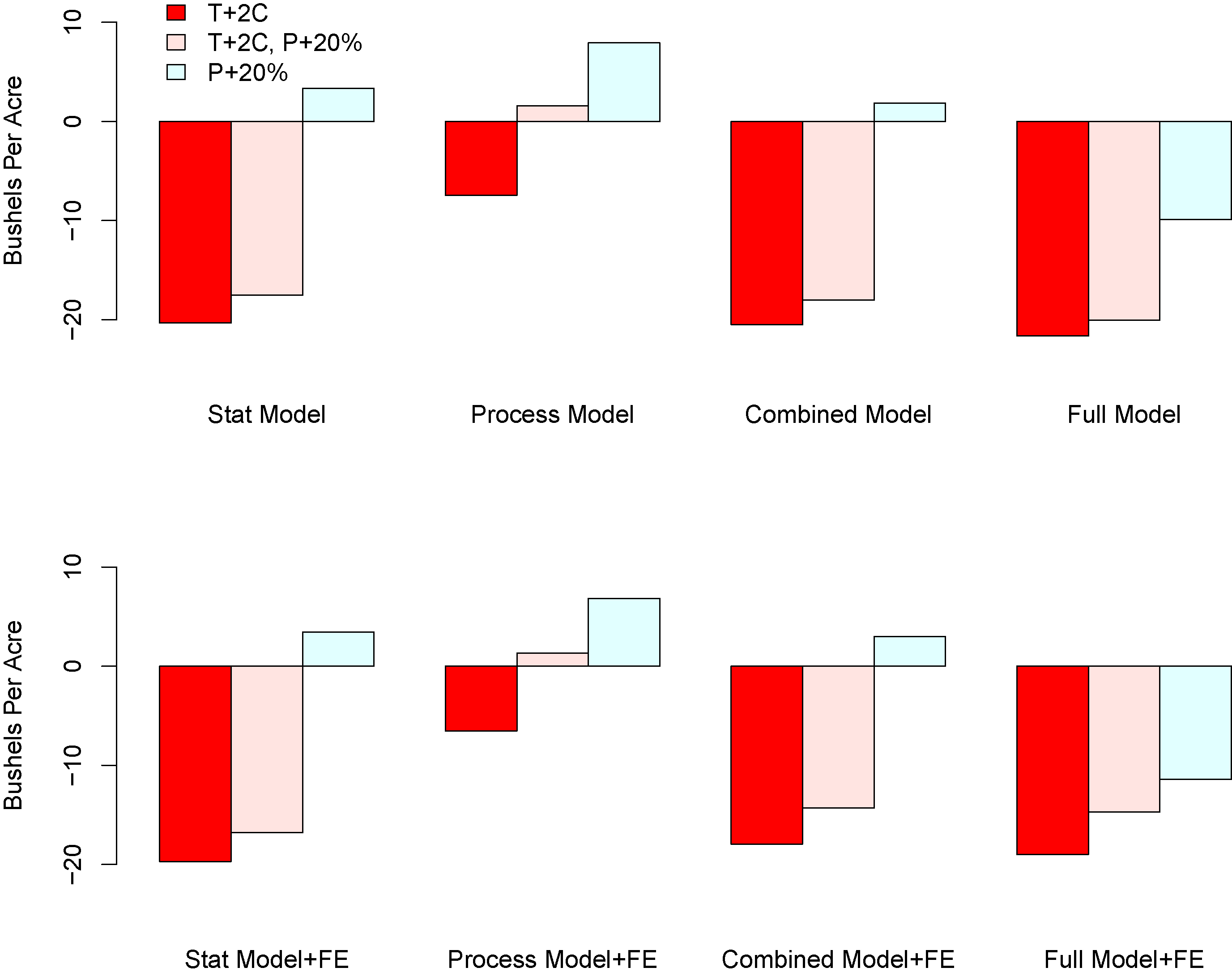
Standard image High-resolution image4.3. Climate change impacts
Predicted climate change impacts are considerably more severe under the statistical model, combined model and full model as compared to the process model (figures 9 and 10). The difference appears to derive from extreme heat effects not captured by the process model (figures 8, 9 and 10). This effect can be seen in a few ways. First, in table 1, the coefficient on HDD, while somewhat smaller in the combined model than in the statistical model, remains substantial in size and and has strong statistical significance. Second, also in table 1, the coefficient on HDD in the emulator models, (j) and (k), though significant, is considerably smaller than both the statistical model and the combined model. These results indicate that the process model cannot account entirely for the association of yield outcomes with extreme heat. The full model shows similar climate change impacts as the combined and statistical models, but shows more damage from greater rainfall.

Figure 9. Climate impacts for different models and change scenarios. Notes: The graphs show aggregated predicted yield changes (bushels per acre) for each model and each climate scenario. Aggregate outcomes are derived by first averaging predicted field-level changes in each county, and then averaging over counties, weighting each county by average harvested acreage between 1995–2012.
Download figure:
Standard image High-resolution image
Figure 10. Climate impacts for a +2C rise in temperature and +20% rise in rainfall. Notes: The maps show predicted yield changes (bushels per acre) for each county and each model, all for the climate change scenario with both an increase in temperature (uniform +2 °C) and increase in precipitation (uniform +20%). The top, middle and bottom rows show impacts for the statistical model, the process model and the combined model, respectively. The left column shows predictions from models without county fixed effects (regressions (a) through (c)) and the right column shows predictions from models with fixed effects (regressions (e) through (g)).
Download figure:
Standard image High-resolution image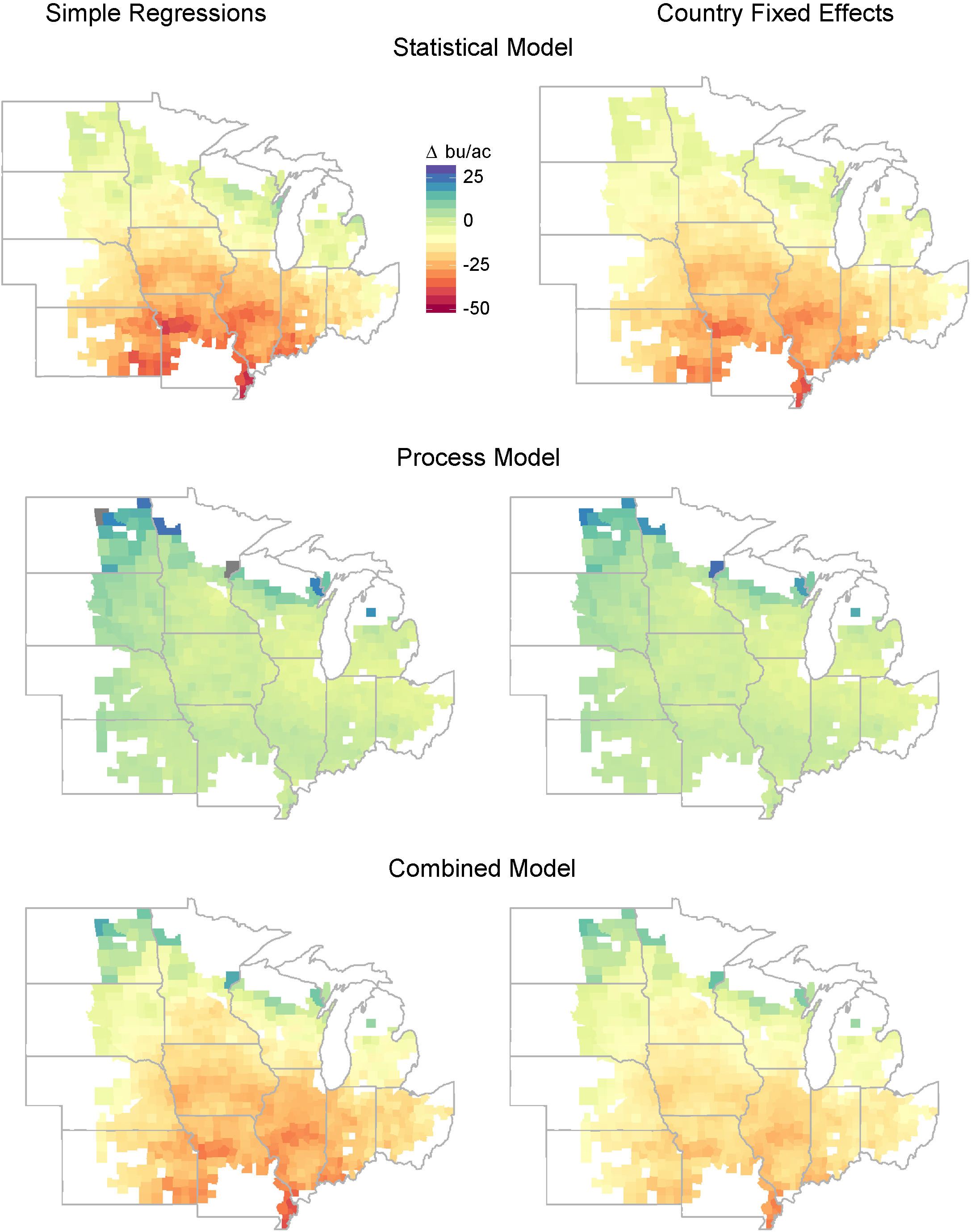
Because models with county fixed effects have predicted damages from climate change that are similar to and often less than those without fixed effects, the statistical and combined models suggest no clear attenuating effects from adaptation. We draw this inference from the fact that identification in regressions with fixed effects comes primarily from year-to-year weather variation, which leaves little account for adaptation, while regressions without fixed effects also draw heavily on the cross-section, which has large differences in climate as well as weather. Thus, holding all else the same, a strong adaptation effect would manifest in more negative impacts with fixed effects than without; we find the opposite. An important caveat to this conclusion is that unobserved factors, like soil depth, may be associated with climate and bias estimates without county fixed effects.
5. Discussion
There has been some debate about whether observed associations between crop yields and extreme heat embody effects of unobserved rainfall, associated lack of soil moisture or other temperature-related effects. Earlier research demonstrates that our measure of extreme heat (HDD) is strongly associated with vapor pressure deficit during critical months of the growing season, which suggests a connection to soil moisture (Roberts et al 2012). Some modeling indicates that low-humidity, high-evapotranspiration events highly correlated with our measure of extreme heat can cause yield loss from water stress in a process-based model similar to the one we employ here (Lobell et al 2013). The research presented here explores this issue in a more comprehensive manner, by explicitly modeling water balance, evapotranspiration and crop growth, and using a combined model to test whether the aggregated weather variables like extreme heat (HDD) possess explanatory power conditional on the process model. We conducted this modeling effort on a vast scale of representative, farmer-managed fields instead of experiment stations.
The results show that both process-model yields and actual yields are negatively associated with extreme heat conditional on rainfall aggregates, but that actual yields are more sensitive to extreme heat than are process-model yields. These results do not necessarily rule out the possibility that observed extreme-heat sensitivity reflects latent drought stress. The cause of the excess sensitivity to extreme heat is not entirely clear. One possibility is that the water balance model and account of soils and root growth in the SSM may be insufficient to accurately account for soil moisture, and that effects of extreme heat may proxy for these inaccuracies in the regression analysis. While the the SSM used in this analysis has many similarities to the APSIM model used in Lobell et al (2013), it may differ with regard to some details of root growth and water balance. Another possibility is that extreme heat, including small exposures to extremes well above 29 °C, cause direct damage, and HDD accounts for this damage and perhaps other effects, like pest damage (Porter et al 1991). Regardless, the results do verify that the extreme heat effect, whatever it may embody physiologically, is substantial, and may be difficult to capture entirely using simple process-based models. The matter deserves more study.
Given the general similarity and high correlation of the predictions, it is interesting that the two models project very different impacts from climate change. While we think these differences deserve further research, we also do not think it is appropriate to conclude that statistical models generally imply greater damages from climate change than do process models. It is worthwhile considering a wider set of models (Lobell and Asseng 2017).
Beyond these particular findings, we have presented a framework for comparing and combining crop models that can improve prediction, help to clarify differences between models, and may ultimately improve assumptions used in crop modeling and ascertaining potential impacts from climate change. The literature is replete with alternative process models and alternative methods and specifications of statistical models (Ben-Ari et al 2016, Sharif et al 2017, Schauberger et al 2017, Lobell et al 2014, Tack et al 2015). The two models we have chosen to investigate here are relatively simple, canonical examples of each type. The same methods could be used to compare and combine multiple models, not just these two. Modern machine-learning and shrinkage estimators could be used to pare redundancies and exploit predictive differences between models. The effect would be similar in spirit to model averaging, but would select weights on competing models (and, implicitly, their underlying assumptions) depending on the degree to which they fit the facts. The approach shares a kindred spirit with the Agricultural Model Intercomparison and Improvement Project (Rosenzweig et al 2013).
Footnotes
- 7
By 'validation' we do not mean 'prove the underlying theory true,' but rather show that the models can successfully predict outcomes in environments outside that in which the model was calibrated.
Supplementary data. (237 KB, PDF)