

Abstract
This study is based on both the recent and the predicted twenty first century climatic and hydrological changes over the mountainous Upper Indus Basin (UIB), which are influenced by snow and glacier melting. Conformal-Cubic Atmospheric Model (CCAM) data for the periods 1976–2005, 2006–2035, 2041–2070, and 2071–2100 with RCP4.5 and RCP8.5; and Regional Climate Model (RegCM) data for the periods of 2041–2050 and 2071–2080 with RCP8.5 are used for climatic projection and, after bias correction, the same data are used as an input to the University of British Columbia (UBC) hydrological model for river flow projections. The projections of all of the future periods were compared with the results of 1976–2005 and with each other. Projections of future changes show a consistent increase in air temperature and precipitation. However, temperature and precipitation increase is relatively slow during 2071–2100 in contrast with 2041–2070. Northern parts are more likely to experience an increase in precipitation and temperature in comparison to the southern parts. A higher increase in temperature is projected during spring and winter over southern parts and during summer over northern parts. Moreover, the increase in minimum temperature is larger in both scenarios for all future periods. Future river flow is projected by both models to increase in the twenty first century (CCAM and RegCM) in both scenarios. However, the rate of increase is larger during the first half while it is relatively small in the second half of the twenty first century in RCP4.5. The possible reason for high river flow during the first half of the twenty first century is the large increase in temperature, which may cause faster melting of snow, while in the last half of the century there is a decreasing trend in river flow, precipitation, and temperature (2071–2100) in comparison to 2041–2070 for RCP4.5. Generally, for all future periods, the percentage of increased river flow is larger in winter than in summer, while quantitatively large river flow was projected, particularly during the summer monsoon. Due to high river flow and increase in precipitation in UIB, water availability is likely to be increased in the twenty first century and this may sustain water demands.
Export citation and abstract BibTeX RIS

Content from this work may be used under the terms of the Creative Commons Attribution 3.0 licence. Any further distribution of this work must maintain attribution to the author(s) and the title of the work, journal citation and DOI.
Corrections were made to this article on 4 February 2015. The first author's email address was corrected.
1. Introduction
Global temperature has increased by 0.72 °C over the period 1951–2012. The projected temperature is likely to increase around 1 °C to 3 °C by 2050s and 2 °C to 5 °C by the end of twenty first century, based on different emission scenarios (IPCC 2013). The increasing rate of warming is significantly higher in the Hindu Kush Himalayan (HKH) region than the global average in the past century (Du et al 2004). Although the Upper Indus Basin (UIB) temperature shows a strong winter temperature increase, it also shows a decrease in summer temperature for some regions (Fowler and Archer 2006, Khattak et al 2011). The warming influence is much higher in the Eastern Himalayas compared with the Greater Himalayan region (Sheikh et al 2014). These temperature variations can have a potential impact on water resources of the UIB and the dependent downstream irrigation demand areas, which are of great concern.
Continuous melting of the glaciers in the Himalayan region may result in severe flooding within the next two to three decades. Receding glaciers will be followed by decreased river flows (Parry et al 2007). An increase of 1 °C in the temperature of UIB would result an increase of 16–17% in summer runoff (Archer 2003). This may also occur at a much higher rate in high-altitude regions than in low-altitude regions since warming is influenced by elevation (Kulkarni et al 2013, Madhura et al 2014). The seasonal mean minimum temperature has significantly increased over the Western Himalaya (Kothawale and Revadekar et al 2010). Pakistan has observed an increased flood risk in recent decades, especially consecutive flooding in the last four years from 2010 to 2013, which affected millions of people, the economy, and the government's infrastructure plans. The Indus River is the major river in Pakistan. It originates in the Himalayas and more than 60% of its river flow comes from snow and glacier melt (Immerzeel et al 2010, Archer and Fowler 2004, Bookhagen and Burbank 2010), which may affect the river flow dynamics of the whole region.
There are few meteorological stations in UIB (Archer et al 2010), thus the use of climate model data in a hydrological model is one of the alternatives for use in such an uphill domain. Many studies have used coarse resolution GCMs' output as an input to a hydrological model in order to analyze the effects of future climate change on water resources (Wilby et al 2008, Goulden et al 2009, Allamano et al 2009). However, the coarse horizontal resolution is not able to delineate reliable climatic projections at a regional scale due to the topography (Fu et al 2008). Dynamically downscaled data can also be used as an input to hydrological models in areas that lack observational data, like the UIB (Akhtar et al 2008). Still, it involves several uncertainties, such as lateral boundary, horizontal resolution and parameterization schemes, which may cause systematic bias in the model output. Such biases lead to unrealistic hydrological results and need to be corrected before being used for hydrological models (Wilby et al 2000). The Karakoram-Himalaya area is still only poorly known, and it has a large variety of climatic conditions and glacier characteristics (IPCC 2013). For such data scarce regions, a hydrological study is a challenging job. Extensive future research is required to increase the reliability of climatic and hydrological projections over mountainous river basins such as the UIB.
The objective of this paper is to examine climatic and hydrological changes over the UIB in recent decades (1976–2005) and future projections (2006–2035, 2041–2070, and 2071–2100). This paper is divided into several different sections. Section 1 provides an introduction and overview of the research study. Section 2 provides information about the study area. Section 3 discusses the data, models, and methodology, including bias correction and calibration of the models. Section 4 presents the results of climatic and hydrological projections, along with limitation and uncertainties in the study. Section 5 concludes the paper and it will also provide some discussion of the topic.
2. Study area
The Indus River is one of the longest rivers and major water carriers in Pakistan, with a total length of 1976 miles (3180 km). It originates from the mountains of the Tibetan Plateau, China and heads toward northern Pakistan. It then diverts southward and flows through the entire length of Pakistan and falls into the Arabian Sea.
The Tarbela dam is a major controlling reservoir which stores the water from the Indus River Basin. The study area, extending from 72°–76°E and 34°N–37°N, upstream of the Tarbela dam is called the UIB (figure 1). The UIB covers upto 164 850 Km2 (Khan et al 2014). Around ∼18 500 Km2 of the total area is covered with glaciers, which significantly contributes to the major runoff of the Indus River from high elevations (Hewitt 2005). Snow melt and glacier melt yield collectively account more than 70% of UIB stream-flows. Most parts of the UIB lie above 5000 meters and it contains the second-highest peak in the world: the K2 Mountain, which is above 8000 meters. Most of the annual precipitation in UIB falls during winter and spring (December-April, DJFMA) due to western disturbances; that is, eastward propagating synoptic systems that are embedded into a westerly flow (Madhura et al 2014). However, the summer monsoon and local circulations only account for one third of the annual precipitation (Young and Hewitt 1990). The climatic conditions of UIB are different from other regions of the country: the monsoon circulation weakens towards northwest in UIB, where the high mountains of the Himalaya decrease the effect of the monsoon circulation. Although the lower elevation stations do not record very high precipitation during winter and summer, the high altitude stations usually record much higher precipitation. Previous studies have suggested a very significant precipitation gradient at high altitudes, and at some parts (>5000 meters) of the basin the annual precipitation exceeds 2000 mm (Mukhopadhyay and Khan 2014). Fowler and Archer (2006) have reported an increasing trend over the past century in both precipitation and temperature during winter, while there is a cooling in summer temperatures. The average river flow to the Tarbela reservoir at Besham Qila reaches 2425 cumecs (cubic meters per second), with a variation of between 80% to 130% from the mean. There are eight meteorological observatories (Kakul, Garidupatta, Balakot, Astor, Bunji, Skardu, Gilgit, and Gupis) in the study area, which are operated by the Pakistan Meteorological Department (PMD). The details of these stations are represented in figure 1 upper and table 8 (below).
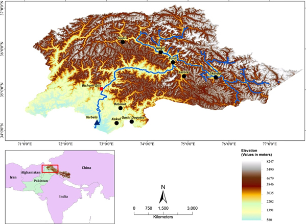
Figure 1. The upper box shows Upper Indus Basin Rivers (blue lines), the Tarbela dam (triangle), Besham Qilla (rectangle), and stations (circles), along with topography. The red color rectangle inside the lower left box shows the location of the study area.
Download figure:
Standard image High-resolution image3. Data and methods
3.1. Data
Daily meteorological observed station data for the period 1976–2010 of maximum temperature, minimum temperature, and precipitation were acquired from the Pakistan Meteorological Department (PMD). This data set were further utilized for the calibration and validation of a University of British Columbia (UBC) model for 1995–2004 and 1990–1994, respectively, and for bias correction of the climate model's precipitation and temperature time series for the period of 1976–2005.
An observed river flow data for the period of 1990–2004 from Besham Qilla gauging station, which is located 80 kilometers (Km) upstream of the Tarbela reservoir, was acquired from the Water and Power Development Authority (WAPDA), Pakistan. This data are sub-divided into two parts (1995–2004 and 1990–1994), and they are used for calibration and validation of the hydrological model. For the simulation of river flow, the UBC model has the limitation of (not more than) five meteorological stations data and one river flow data. We have eight meteorological stations; therefore, to make a total of five meteorological stations, the data are aggregated by averaging two stations nearest to each other. The averaging criterion is based on the closeness of latitude, longitude, and elevation of the stations. The detail of the meteorological stations is given in table 8.
The output data of climate models for the period 1976–2005, 2006–2035, 2041–2070, and 2071–2100 of CCAM and 2041–2050 and 2071–2080 of RegCM were also used for the extraction of the time series of temperature and precipitation for the corresponding location of meteorological stations. These data were used to compare with observed station data for the purpose of bias correction and then used as an input to the hydrological model to acquire the future river flow projection. The resolution of these data is 50 km and 60 km, respectively. The climate model's output datasets are based on future emission scenarios of the Representative Concentration Pathways (RCP) (van Vuuren et al 2011), RCP4.5 (Clarke et al 2007) with 4.5 W m−2, and RCP8.5 (Riahi et al 2007) with 8.5 W m−2 radiative forcing by 2100.
Climate Research Unit (CRU TS3.10, Harris et al 2014) data are used for the general graphical representation of mean seasonal variation, along with the climate model's data. These data includes monthly mean temperature and precipitation for the time period of 1976–2005 over the land at regular global 0.5 degree intervals.
3.2. A Description of the numerical models
3.2.1. CCAM
The output of the Conformal-Cubic Atmospheric Model (CCAM) is used as an input to the hydrological model in this study. A global variable resolution model CCAM was developed at CSIRO, Australia. It was designed for regional climate downscaling and atmospheric climate modeling (McGregor and Dix 2001). CCAM is able to simulate the regional atmospheric conditions in contrast to the limited-area models, by using a stretched conformal cubic grid while focusing on the area of interest (McGregor 2005). The CCAM has been integrated from coarse resolution (200 km) to a much higher resolution (15 km), and this has resulted in considerably more specific and accurate forecasts. The results of inter-comparison project of many models show that CCAM is a good model to reproduce the climatic features of Southeast Asia (Fu et al 2005).
3.2.2. RegCM
The output of RegCM is also used as an input to the hydrological model in this study. The first version of RCM was developed during the 1980s (Dickinson et al 1989). Since then newer versions have been introduced, as RegCM2 and RegCM3 (Giorgi et al 1993, Pal et al 2000, 2007). The latest version is RegCM4, which is maintained by 'Earth System Physics' (ESP), Abdul Salam International Center for Theoretical Physics (ICTP), Italy (Giorgi et al 2012). RegCM4 is more flexible, user friendly, and portable, involving the ease for necessary updates in source code. The dynamic core of this version is very similar to the previous version (RegCM3), which was based on hydrostatic version of the NCAR/Penn State meso-scale model MM5 (Grell et al 1994). The radiation scheme of the modified NCAR Community Climate Model version 3 (CCM3; Kiehl et al 1998) is used. The Biosphere-Atmosphere Transfer Scheme (BATS) is used as the land-surface model (Dickinson et al 1993). Holtslag et al 1990 scheme has parameterized the Planetary Boundary Layer (PBL) computations. The SUBEX scheme represents the resolvable scale precipitation (Pal et al 2000). The development of a non-hydrostatic dynamical core, and coupling with regional ocean model and physics schemes (cloud microphysics, convection, PBL) are under process. Giorgi et al (2012) has discussed the physical processes and parameterization of RegCM4 in detail.
3.2.3. UBC watershed hydrological model
In this study, the UBC hydrological model is used to generate the projection of the river's future flow at the Tarbela reservoir. This model was developed in 1973 especially for the calculation of stream flow over mountainous regions. It has also been used in studies for the projections of hydrological processes due to climate change (Merritte et al 2006). This model has also been used in different studies in British Columbia specifically for the Columbia River system, the UIB River in Pakistan, and the Saskatchewan River system in Alberta (Quick and Pipes 1977, Naeem et al 2013). This model is divided in three sub models: the meteorological module, the soil moisture module, and the module related to routing of the runoff, which is described by Quick and Pipes (1977). The meteorological component distributes the point values of temperature and precipitation ranges to several elevation bands of the watershed. The changes in temperature with altitude control the precipitation fall rate as snow or rain and the melting of snow. The soil moisture module represents the non-linear response of the watershed and is further divided into four parts, which are: extremely slow runoff in the deep ground water, slow runoff in the upper ground water, fast runoff at the surface, and medium runoff as an interflow. The runoff routing module permits the release of runoff to the watershed outlets. This is based on the theory of a linear reservoir that assumes the water equilibrium and conservation of mass. The daily dataset of river flow, precipitation, minimum, and maximum temperature are used as the input to the UBC hydrological model.
3.2.4. Snowmelt module in the models
Use of climate model outputs as an input to the hydrological model without consideration of glacier responses to climate change and hydrological impacts studies in the Himalayan high mountains is still an unanswerable question. All three models of GCM, RCM and hydrological model used in our study handle the snowmelt. However, these models did not include a comprehensive parametrization of glaciers, more work particularly related to glacier melting is required.
The UBC hydrological model is specially developed for use in mountainous regions. In such regions, the data on higher elevations are usually scarce. The UBC divides these regions into different bands, and interpolates the data of temperature and precipitation through the lapse rate over the whole region where there is no observed data available. The model operates continuously, accumulating and depleting the snowpack and producing inflow. For snowmelt estimation, UBC uses an energy budget approach that requires radiation, cloud cover, albedo, wind, cloud temperature and dew point temperature data. Usually, in high mountainous regions these data are not available. The model calculates the values of these data using temperature based equations.
CCAM predicts its own snow cover and associated runoff like other GCMs, such as ACCESS, HadGEM, GFDL, and CSIRO Mk3.6. Soil texture (e.g., clay, loam, silt, etc) is specified for each grid point and some points have the soil texture specified as permanent ice. This means that the soil parameters will be set to ice values, which affects the thermal conductivity, etc. Energy is still conserved and the prognostic snow on top of the soil will still evolve as normal (i.e., not as prescribed). The term glacier is a bit confusing in the model and CCAM does not explicitly model glaciers. The CCAM can produce some fairly large snow depths if it accumulates a lot of precipitation without any chance for melting due to cold temperatures. If this happens and the snow depth becomes too large, then the snow depth is limited to a maximum amount but the temperature is adjusted so that the total energy budget is still conserved. Points where the snow depth has become limited are referred to as glaciers but this does not mean that these points correspond to real glaciers. In a hydrological budget the water undergoes phase transitions between vapors, liquid, and ice, as described by the cloud microphysics and the convection processes simulated by the model. The land surface model conserves both energy and water within the column through its prognostic equations describing the physics of the canopy, soil, snow, etc.
In RegCM glaciers are also not present. There is no estimation of the water stored in glacier reservoirs. RegCM initializes snow cover, beginning with an estimation of the glacier's water content in the initial snow cover depth, but correct modelling of ice melting would require the addition of a glaciology model. As it is now, the model would consider that snow and melt it using a simple temperature/snow age driven function. Snow fall and melting is consistent and the model can handle it. The local water budget is missing the river transport; that is, the model has just local runoff and does not have water transport by rivers. Consequently, evaporation may not take place in the correct location. In addition, irrigation is not present, albeit no one has yet gone into evaluating the CLM4.5 capabilities on this.
3.3. Methodology
The first phase (phase 1) is based on the CCAM output with RCP4.5 and RCP8.5 lateral boundary conditions (LBC) from the global model (MPI ESM) for the period of 1976–2005 as a baseline and 2006–2035, 2041–2070, and 2071–2100 as future periods. In the second phase (phase 2), we first take the RegCM model output for 2041–2050 and 2071–2080 with RCP8.5 LBC from MPI ESM and second take the 2071–2080 with RCP8.5 and RCP4.5 LBC from Geophysical Fluid Dynamics Laboratory (GFDL). The time slice of RegCM output is decadal (10 years each) and less than that of CCAM (30 years each). However, the RegCM time slices are in the period range of CCAM and are comparable. The main consideration and discussion of this study is based on the results of phase 1. The results of the second phase (phase 2) are only used for a general comparison of the two different models (CCAM and RegCM). To minimize the differences between the actual climate (observed) and model (CCAM) data, the model simulation for 1976–2005 was first compared with observed station data and then the biases were corrected using Best Easy Systematic (BES, Wonnacott and Wonnacott 1972) and Mean Monthly Correction Factor (MMCF) statistical methods. The same bias correction assumption is then applied to model data for future periods of 2006–2035, 2041–2070, and 2071–2100. The same process is repeated for RegCM data. The hydrological model was first calibrated and validated with observed meteorological data and observed river flow data, before applying bias-corrected data as an input for the future hydrological projections. The general methodology of this work is demonstrated graphically in figure 2.

Figure 2. Methodology flow chart for the future climatic and hydrological projection over the UIB with CCAM output on 50 km for the periods (1976–2005, 2006–2035, 2041–2070 and 2071–2100) with RCP4.5, RCP8.5, and RegCM outputs on 50 km for the periods (2041–2050 and 2071–2080) with RCP4.5 and RCP8.5. Observed metrological station (1976–2005) and observed river flow (1990–2004) data are used for bias correction of the climate model's output, and for validation and calibration of the hydrological model. The bias corrected data are used for future climatic change projection and as an input to the hydrological model for future hydrological projection.
Download figure:
Standard image High-resolution image3.3.1. Bias correction
The dynamically downscaled data could lead to unrealistic hydrological results without the application of bias correction (Akhtar et al 2008, Bergstrom et al 2001, Graham et al 2007, Haerter et al 2011). Statistical bias correction corrects the biases in the simulated climate time series corresponding to the observed time series. The process of bias correction typically preserves the difference (climate change signal) between baseline (e.g. 1976–2005) and future periods (e.g. 2006–2035, 2041–2070, and 2071–2100). There are several methods to implement bias correction. First, the Best Easy Systematic (BES) (Wonnacott and Wonnacott 1972) estimator is used for both temperature and precipitation. Although the BES method is good for temperature, its performance is low for precipitation. Afterwards, the Mean Monthly Correction Factor (MMCF) method is used for precipitation bias correction.
According to Woodcock and Engel 2005, among linear methods, the BES method is better to compute because it is a robust technique and is simple to apply. Mathematically the BES estimator is represented as:

The first, second, and third quartiles of the bias series between simulated and observed data are represented by Q1, Q2, and Q3. BES is used for future data and is basically computed for the baseline data. The difference of BES estimator and RCM's output data are calculated at the end to avoid bias. The MMCF method was computed for bias correction of already downscaled precipitation data. The MMCF method has been extensively used in many studies (Teutschbein and Seibert 2010, Lafon et al 2012).
The transformed precipitation is given by the relation:

The model's daily output precipitation after the bias correction is represented by R*, R is the model's daily output precipitation before the application of bias correction technique, and the mean monthly correction factor is represented by k and is calculated by:
3.3.2. Calibration and validation of the UBC model
Calibration of the hydrological model is an important step because the model cannot be directly used for a basin wide study without calibration (Schuol and Abbaspour 2006, Haerter et al 2011). In calibration, the observed daily station data of temperature and precipitation are used as an input to the hydrological model and the model river flow is compared with the observed daily river flows. The sensitive parameters of precipitation gradient factors (P0GRADL, P0GRADM and P0GRADL), adjustment to precipitation (P0GRADL and P0RREP), groundwater percolation (P0PERC), fraction of impermeable area in the band (C0IMPA), groundwater percolation (P0PERC), deep zone share fraction (P0DZSH), time constant for upper groundwater runoff (P0UGTK), and time constant for deep groundwater runoff (P0DZTK) are tuned for future river flow projections. The performance of the model was statistically validated against the Nash-Sutcliffe coefficient of efficiency (CE). This method is usually applied to the calibration of a hydrological model (Bardossy 2007, Shi et al 2008, Westerberg et al 2011). The statistical equation for this method is given below:
where,

n represents the total timestep numbers, Qoi represents the observed water flow of ith timestep, whereas Qsi represents the simulated water flow of ith
The other calculations involved in this study to evaluate the simulated change in water river flow (R2) are represented by the following equations.
Where,
The model perfectly captures the observed river flow pattern if the value of Ceff is equal to one. If the value of R2 approaches to one, then the observed river flow is perfectly captured by the model. R2 is the correlation coefficient used for comparison of the time and shape of the simulated river flow's hydrograph with the observed river flow. Ceff tells how accurate the estimated hydrographs' volume, time, and shape is to that of the observed hydrograph.
4. Results and discussion
4.1. Climatic changes
UIB climate varies significantly over time and space due to its complex topography, weaker summer monsoon, and higher rainfall during winter and early spring due to western disturbances. These characteristics make this region distinct from other regions in South Asia.
Figure 3 shows the seasonal mean air temperature of CCAM for 1976–2005, 2006–2035, 2041–2070, and 2071–2100 along with CRU for 1976–2005. The model surface air temperature during 1976–2005 is generally in agreement with CRU for seasonal variations. However, there are some biases that underestimate the temperature, such as the summer simulation to east of 76°E. Furthermore, the southern areas, which are dominated by the summer monsoon, show a smaller difference with some overestimation than the northern parts where the difference is larger and underestimated. The same phenomena are also found when the results of the model were compared with the station observed data. This indicates that the model's performance is passive at the northern parts and shares the common problem of cold biases over UIB, which exists throughout the year (tables 1–2). The possible reason for the cold bias may be: (1) the difference in elevation between the model and actual station values; or, (2) the sudden variation in the topography of this mountainous region, such as the windward and leeward problem. The model's results also show warming during spring as well as in winter for the whole period. The monthly seasonal mean of maximum temperature and difference of temperature from the baseline (1976–2005) to the future (2006–2035, 2041–2070, 2071–2100) is shown in tables 1 and 2. In RCP8.5, the increase in temperature for 2006–2035 is 2.2 °C, for 2041–2070 it is 4.2 °C, and for 2071–2100 it is 5.8 °C. In RCP4.5 the increase in temperature for 2006–2035 is 0.5 °C, for 2041–2070 it is 1.5 °C, and for 2071–2100 it is 2.0 °C. The increase in minimum temperature is high in both scenarios for all future periods, which is an important parameter for the sustainability and growth of agriculture in the region. The temperature increase is higher in the spring (MAM) and winter (DJF) than in the summer (JJA), except in the northern parts where the increase in summer temperature is higher in RCP8.5. A comparison of RCP8.5 and RCP4.5 shows that the average temperature increase is more than double in RCP8.5 than RCP4.5. It is very important to note that in RCP4.5 the temperature increase is relatively slow in 2071–2100 as compared to 2041–2070. The RegCM results also show an increase in future temperature and are in agreement with CCAM results. During 2041–2050 the increase in minimum temperature is 1.7 °C and the maximum temperature is 1.9 °C. For the period 2071–2080, the increase in minimum and maximum temperature is 4.3 °C and 4.4 °C, respectively, whereas the total increase in temperature is 1.8 °C and 4.3 °C for 2041–2050 and 2071–2080 periods, respectively. In RegCM, the average temperature increase is more in RCP8.5 than RCP4.5. The temperature increase is higher in spring (MAM) and winter (DJF) as compared to summer (JJA). Thus, the results provide evidence that there are significant changes in maximum and minimum temperatures in both models with RCPs, which indicate the signals of future climatic change over UIB.
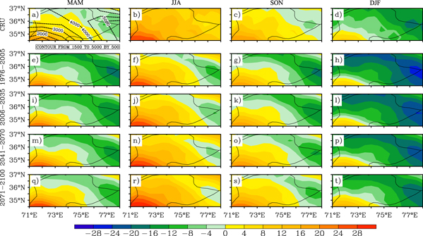
Figure 3. Seasonal mean temperature of MAM ((a), (e), (i), (m), (q)), JJA ((b), (f), (j), (n), (r)), SON ((c), (g), (k), (o), (s)) and DJF ((d), (h), (l), (p), (t)) of CRU and CCAM with emission scenario RCP8.5 (units: °C). The dashed lines in (a) indicate the elevation. (unit: m).
Download figure:
Standard image High-resolution imageTable 1. Seasonal mean (upper) and future increase (lower) in minimum, maximum temperature for the observation from metrological stations over UIB (1976–2005) and CCAM 1976–2005, 2006–2035, 2041–2070, 2071–2100 with RCP8.5 (units: °C).
| Seasonal mean of max-temperature | Seasonal mean of min-temperature | ||||||||
|---|---|---|---|---|---|---|---|---|---|
| Duration | DJF | MAM | JJA | SON | DJF | MAM | JJA | SON | Average |
| Observation | 8.5 | 20.6 | 30.2 | 21.1 | −1.3 | 9.4 | 18.1 | 7.9 | 14.9 |
| 1976–2005 | 2.5 | 15.1 | 22.2 | 12.2 | −9.1 | 2.0 | 8.6 | 1.0 | 7.5 |
| 2006–2035 | 3.4 | 16.2 | 23.3 | 13.0 | −5.5 | 5.9 | 12.4 | 4.1 | 9.6 |
| 2041–2070 | 5.5 | 18.3 | 25.4 | 15.0 | −3.4 | 7.7 | 14.2 | 5.9 | 11.6 |
| 2071–2100 | 8.3 | 21.5 | 28.7 | 17.2 | −2.4 | 7.9 | 14.0 | 6.2 | 13.4 |
| Future increase in max-temperature with 1976–2005 | Future increase in min-temperature with 1976–2005 | ||||||||
| 2006–2035 | 0.8 | 1.1 | 1.1 | 0.7 | 3.5 | 3.9 | 3.8 | 3.0 | 2.2 |
| 2041–2070 | 2.9 | 3.1 | 3.2 | 2.7 | 5.6 | 5.7 | 5.6 | 4.9 | 4.2 |
| 2071–2100 | 5.8 | 6.3 | 6.4 | 5.0 | 6.7 | 5.9 | 5.4 | 5.1 | 5.8 |
Table 2. Same as table 1 but for RCP4.5.
| Seasonal mean of mMax-temperature | Seasonal mean of min-temperature | ||||||||
|---|---|---|---|---|---|---|---|---|---|
| Duration | DJF | MAM | JJA | SON | DJF | MAM | JJA | SON | Average |
| Observation | 8.5 | 20.6 | 30.2 | 21.1 | −1.4 | 9.2 | 18.0 | 8.3 | 14.3 |
| 1976–2005 | 2.9 | 15.5 | 23.0 | 12.8 | −9.0 | 1.6 | 8.6 | 1.3 | 7.1 |
| 2006–2035 | 3.2 | 16.2 | 23.1 | 12.7 | −8.7 | 3.0 | 9.6 | 2.1 | 7.6 |
| 2041–2070 | 4.4 | 17.0 | 24.2 | 13.7 | −7.1 | 3.6 | 10.2 | 3.1 | 8.6 |
| 2071–2100 | 4.8 | 17.6 | 24.9 | 14.1 | −6.6 | 4.3 | 10.8 | 3.5 | 9.2 |
| Future increase in max-temperature with 1976–2005 | Future increase in min-temperature with 1976–2005 | ||||||||
| 2006–2035 | 0.2 | 0.6 | 0.0 | −0.0 | 0.3 | 1.3 | 0.9 | 0.7 | 0.5 |
| 2041–2070 | 1.4 | 1.5 | 1.1 | 0.9 | 1.9 | 1.9 | 1.6 | 1.7 | 1.5 |
| 2071–2100 | 1.8 | 2.0 | 1.8 | 1.3 | 2.4 | 2.6 | 2.2 | 2.2 | 2.0 |
Figure 4 illustrates seasonal mean precipitation of CCAM for 1976–2005, 2006–2035, 2041–2070, and 2071–2100. It is found that CCAM overestimated the precipitation for all the seasons especially in Autumn (SON). There is less precipitation during the summer monsoon season, which indicates a weaker monsoon. Overall the occurrence of precipitation is highly variable, as compared to the consistent temperature increase in this region. The projected precipitation increase in RCP4.5 and RCP8.5 is almost same as the 10–11% for 2006–2035 and the 13% for 2041–2070. For 2071–2100, although there is still a difference between the two RCPs, it continuously increases, with 12% (slightly lower by comparison of 2041–2070) and 20%, respectively (table 3). Projected precipitation by RegCM also shows increasing trends for future time periods, which shows a 14% and 23% increase for 2041–2050 and 2071–2080, respectively. By 2080, the precipitation difference of RCP4.5 and RCP8.5 in RegCM is not very promising. The results from Kulkarni et al (2013) over UIB also show a 20–40% increase in 2071–2098 for summer monsoon precipitation from the baseline period (1961–1990). There is also an increase in the precipitation of meteorological stations of the northern part (i.e. Garidupatta, Astor, Bunji, Skardu, Gilgit, and Gupis) but a decrease in the southern part stations (Kakul and Balakot), particularly in winter.
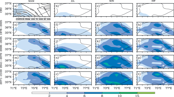
Figure 4. Same as figure 3, but for precipitation (unit: mm day−1).
Download figure:
Standard image High-resolution imageTable 3. Seasonal mean (upper: mm day−1) and future percentage increase (lower: %) values of precipitation for the whole domain of UIB for the observation from metrological stations over UIB (1976–2005) and CCAM 1976–2005, 2006–2035, 2041–2070, 2071–2100 with RCP8.5 and RCP4.5.
| Seasonal values of precipitation in RCP8.5 | Seasonal values of precipitation in RCP4.5 | |||||||||
|---|---|---|---|---|---|---|---|---|---|---|
| Duration | DJF | MAM | JJA | SON | Average | DJF | MAM | JJA | SON | Average |
| Observation | 1.4 | 2.1 | 3.1 | 1.0 | 1.9 | 1.4 | 2.1 | 3.1 | 1.0 | 1.9 |
| 1976–2005 | 2.9 | 2.0 | 4.0 | 4.0 | 3.3 | 2.8 | 2.1 | 4.2 | 3.9 | 3.2 |
| 2006–2035 | 3.1 | 2.3 | 4.4 | 4.7 | 3.6 | 2.6 | 2.2 | 4.8 | 4.8 | 3.6 |
| 2041–2070 | 2.9 | 2.3 | 4.7 | 5.0 | 3.7 | 3.1 | 2.2 | 4.6 | 5.0 | 3.7 |
| 2071–2100 | 3.0 | 2.7 | 4.6 | 5.4 | 3.9 | 2.9 | 2.3 | 4.6 | 5.1 | 3.7 |
| Future percentage increase of precipitation with 1976–2005 in RCP8.5 | Future percentage increase of precipitation with 1976–2005 in RCP4.5 | |||||||||
| 2006–2035 | 7.6 | 11.6 | 8.9 | 16.1 | 11.0% | −5.1 | 8.4 | 14.9 | 21.9 | 10.0% |
| 2041–2070 | −1.2 | 14.2 | 16.1 | 24.5 | 13.4% | 11.5 | 5.7 | 9.4 | 26.6 | 13.3% |
| 2071–2100 | 3.5 | 32.9 | 13.0 | 33.2 | 20.7% | 3.2 | 8.8 | 8.5 | 30.1 | 12.6% |
4.2. Bias correction and calibration
The CCAM model data for the baseline period (1976–2005) is compared with observed station data, and differences between model and observed data are found. To minimize these differences, the statistical techniques of the BES estimator method for temperature and the MMCF method for precipitation is used. The results before and after bias corrections are shown in figures 14–16, which clearly show that: BES is best for temperature bias correction, the performance BES is low for precipitation, while MMCF performance is very good for precipitation. The same bias correction assumptions are applied to 2006–2035, 2041–2070, and 2071–2100. It is clear from the analysis that bias correction methods remarkably minimized the differences between observed and modeled data, which almost overlaps the observed and bias corrected curve. These biases-corrected time series data are used as inputs to the hydrological model for impact assessment.
For calibration and validation, the observed river flow data are divided into two parts: first, 1995–2004 is used to calibrate UBC model; and second, the data from 1990–1994 are used for validation. The model parameters mentioned in the methodology were adjusted for calibration. The results of calibration for 1995–2004 with mean monthly flow of 2320 cumecs and the observed monthly flow of 2470 cumecs are shown in figure 5. The statistical analysis shows the higher efficiency of UBC of 0.9 (Berenguer et al 2005) for the study region using Nash-Sutcliffe statistics. The calibration river flow results of the model are closer to the observed river flow in summer than winter. The calibrated model was also validated before simulation for future projection of river flow for 1990–1994. For validation, the efficiency statistics are even higher than the calibration period.

Figure 5. Calibration of the UBC hydrological model for the years 1995–2004. The observed and simulated river flows are shown by the black and grey line, respectively.
Download figure:
Standard image High-resolution image4.3. Hydrological changes
The bias-corrected outputs of the CCAM and RegCM climate models were used as an input to the calibrated hydrological model for the river flow simulation. For CCAM, simulations of 1976–2005 and projections of 2006–2035, 2041–2070, and 2071–2100 were carried out (based on MPI-ESM with RCP8.5 and RCP4.5). The period of 1976–2005 was considered as a baseline for river flow. The results suggest that total river flow is continuously increasing over time in the Upper Indus River. The increasing rate of river flow in both RCPs is enhanced during the first two time slices (2006–2035 and 2041–2070), while it is smaller and not in the same ratio during the last time slice (2071–2100) in RCP8.5 and it even decreases for RCP4.5 when compared with 2041–2070. In the summer for RCP4.5, the increase is 24% during 2006–2035, 32% during 2041–2070, and 26% during 2071–2100. In RCP8.5, the percentage increase is 23% during 2006–2035, 50% during 2041–2070, and 55% during 2072–2100. The results show that percent increase is higher in winter than summer in both scenarios. Maximum river flow occurring in summer shows that the highest river flow in RCP8.5 is of 9720 cumecs for the period of 2006–2035, 11 837 cumecs for the period of 2041–2070, and 12 222 cumecs for the period of 2071–2100. In RCP4.5 the highest river flow in summer is 9783 cumecs for the period of 2006–2035, 10 428 cumecs for the period of 2041–2070, and 9954 cumecs for the period of 2071–2100. The projection for increased river flow was higher in RCP8.5 than RCP4.5, mainly due to a significant increase in temperatures. The details of mean river flow values input from CCAM are listed in tables 4 and 5, and shown in figures 6(a) and (b). In RegCM, the increase in river flow during summer is 36% in 2041–2050 and 56% during 2071–2080. Maximum river flow occurs in summer and shows the highest rate of river flow, that is: 7327 cumecs for the period of 2001–2010, 8602 cumecs for the period of 2041–2050, and 9926 cumecs for the period of 2071–2080. The average river flow was measured as 2209 cumecs for the period of 2001–2010, 3328 cumecs for the period of 2041–2050, and 4050 cumecs for the period of 2071–2080. The details of mean river flow values input from RegCM are listed in table 6 and shown in figures 6(c) and (d). For both models, the minimum river flow occurs in the months of December-February when river flow is in the range of 70 to 700 cumecs. The percentage increase is higher in winter than in summer. In RegCM, the comparisons of RCP4.5 and RCP8.5 for the future inflow projection with time period 2071–2080 are quite close to each other and show almost similar results in the months of September-May. However, RCP8.5 shows more increase than RCP4.5, with a significant difference in the months of April-August.
Table 4. Mean monthly river flows values (cumecs) of UBC for the period of baseline 1976–2005, and future 2006–2035, 2041–2070, 2071–2100 input from CCAM with RCP4.5 and RCP8.5.
| RCP8.5 | RCP4.5 | ||||||
|---|---|---|---|---|---|---|---|
| Month | Base River flow | 2006–2035 | 2041–2070 | 2071–2100 | 2006–2035 | 2041–2070 | 2071–2100 |
| October | 964 | 1678 | 2037 | 2357 | 1536 | 1787 | 1672 |
| November | 383 | 710 | 807 | 986 | 711 | 815 | 710 |
| December | 279 | 489 | 490 | 508 | 460 | 614 | 433 |
| January | 220 | 425 | 371 | 481 | 393 | 444 | 304 |
| February | 178 | 397 | 427 | 612 | 369 | 473 | 376 |
| March | 231 | 818 | 816 | 1565 | 737 | 858 | 644 |
| April | 878 | 1799 | 2127 | 3711 | 1885 | 1894 | 1866 |
| May | 2752 | 4407 | 6040 | 8686 | 4363 | 5387 | 4487 |
| June | 6839.23 | 8913 | 12 192 | 12 492 | 9387 | 9873 | 9329 |
| July | 9408.98 | 11 458 | 13 279 | 13 171 | 11 464 | 12 072 | 11 686 |
| August | 7289.58 | 8790 | 10 040 | 11 004 | 8497 | 9340 | 8848 |
| September | 3917.74 | 5009 | 5965 | 6778 | 4769 | 5392 | 4779 |
| Average | 2778 | 3741 | 4549 | 5196 | 3714 | 4079 | 3761 |
Table 5. Percent increase (%) in mean of monthly river flows values of UBC for the period of baseline 1976–2005, and future 2006–2035, 2041–2070, 2071–2100 input from CCAM with RCP4.5 and RCP8.5.
| RCP8.5 (% increase river flow) | RCP4.5 (% increase river flow) | |||||
|---|---|---|---|---|---|---|
| Month | 2006–2035 | 2041–2070 | 2071–2100 | 2006–2035 | 2041–2070 | 2071–2100 |
| October | 73 | 111 | 144 | 59 | 85 | 73 |
| November | 85 | 110 | 157 | 85 | 112 | 85 |
| December | 75 | 75 | 81 | 64 | 119 | 55 |
| January | 93 | 68 | 118 | 78 | 101 | 37 |
| February | 122 | 138 | 242 | 106 | 164 | 110 |
| March | 253 | 253 | 576 | 218 | 271 | 178 |
| April | 104 | 142 | 322 | 114 | 115 | 112 |
| May | 60 | 119 | 215 | 58 | 95 | 63 |
| June | 30 | 78 | 82 | 37 | 44 | 36 |
| July | 21 | 41 | 39 | 21 | 28 | 24 |
| August | 20 | 37 | 50 | 16 | 28 | 21 |
| September | 27 | 52 | 73 | 21 | 37 | 22 |
| Average | 34 | 63 | 87 | 33 | 46 | 35 |

Figure 6. River flows simulation of UBC for the period of baseline (1976–2005), projection for 2006–2035, 2041–2070, 2071–2100 with CCAM (for RCP4.5 figure 6(a) and RCP8.5 figure 6(b)) and 2041–2050, 2071–2080 with RegCM (for RCP8.5 figure 6(c) and RCP4.5&85 with GFDL figure 6(d)).
Download figure:
Standard image High-resolution imageTable 6. Mean monthly river flows values (cumecs) and river flow percentage (%) increase of UBC for the period of future one (2041–2050) and future two (2071–2080) ) input from RegCM with RCP4.5 and RCP8.5.
| Month | 204I–2050 RCP8.5_MPI | 2071–2080 RCP8.5_MPI | 2071–2080 RCP4.5_GFDL | 2071–2080 RCP8.5_GFDL | 204I–2050 RCP8.5_MPI% increase | 2071–2080 RCP8.5_MPI% increase |
|---|---|---|---|---|---|---|
| October | 1236 | 1694 | 1210 | 1306 | 122 | 205 |
| November | 474 | 606 | 635 | 576 | 205 | 290 |
| December | 261 | 202 | 374 | 291 | 198 | 131 |
| January | 199 | 569 | 299 | 225 | 180 | 698 |
| February | 198 | 332 | 349 | 204 | 192 | 389 |
| March | 790 | 1059 | 519 | 550 | 394 | 563 |
| April | 1826 | 2442 | 1426 | 1596 | 127 | 204 |
| May | 4893 | 6621 | 3730 | 5148 | 74 | 135 |
| June | 8337 | 10 068 | 9561 | 10 036 | 48 | 78 |
| July | 9581 | 10 370 | 10 599 | 11 478 | 32 | 43 |
| August | 7890 | 9340 | 8931 | 8762 | 29 | 52 |
| September | 4247 | 5297 | 4088 | 4336 | 50 | 87 |
| Average | 3328 | 4050 | 3477 | 3709 | 50% | 83% |
The increase of river flow in winter is mainly due to an increase in precipitation since the contribution from the snow is less because of low temperature (<0 °C) in most parts of UIB. The increasing river flow rate in summer is mainly associated with warming summer temperatures, which causes higher ablation of snow and, in turn, a higher contribution to river flow. The observed river flows from 1990–2000 were also analyzed to find the correlation of river flow with observed minimum, maximum temperatures, and precipitation. Figure 7 shows that maximum temperature and minimum temperature are the main influencing factors and have strong correlation with river flow while precipitation has a weak correlation with river flow, and it even has a negative correlation (−0.38) over the Skardu station. The reason for the negative correlation is that the temperature is mostly below freezing point over this station, and snow and glaciers become deeply frozen and require ripening before melt can occur.
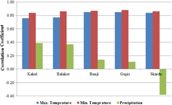
Figure 7. Correlation coefficient between observed metrological variables [maximum temperature (blue bar), minimum temperature (red bar), and precipitation (green bar)] with observed river flow for the period (1991–2000) over different stations.
Download figure:
Standard image High-resolution imageThe patterns of temporal changes in the river flow for the future periods are similar but different in magnitude. Chaturvedi et al (2014) has stated that an increased glacial retreat is expected in many sub-regions of the Karakoram-Himalayan region. The glaciers of this region are projected to lose a mass of larger than 1200 kgm−2a−1. About 13% glacial area in the Western Himalaya region, 10% in Central Himalaya region, and 34% in the Eastern Himalaya region will have melted by 2030, as projected by RCP8.5, or by 2080, as projected by RCP26. Our findings for river flow are in accord with the results of recent study of Immerzeel et al (2013) that conclude consistent increase (300%) of river flow with RCP8.5 from one selected glacier in UIB during the twenty first century. Our results for RCP8.5 show that the total increase of river flow is about 87%, which is less than the findings of Immerzeel et al (2013) and this may be due to their consideration of only one glacier to estimate future river flows. In our study we represent the whole UIB area, where the area covered by glaciers is not more than 12% of the entire basin and the whole basin area would not contribute to the river flow, therefore our results seem reasonable.
The results of the present study are in accordance with the IPCC report AR4 (IPCC 2007) and future projections on the feedback of global climate change over glacierized basins (Rees and Collins 2006), which says that in first half of twenty first century a short-term increase in river flow is expected while in the last half of twenty first century there may be a sharp decrease in river flow. The results of both models indicate a rising trend with a higher increase in the rate of the river flow in the first half of the century. Meanwhile, the increasing rate is comparatively low in the last half of the twenty first century in RCP4.5 for 2071–2100, which may possibly be due to: (1) a persistent decrease in overall basin snow cover area, and (2) a slight lowering in warming and precipitation trends in RCP4.5 during that period, which might imply relatively less snow ablation and which in turn reduces the river flow. However, in the second case, the lowering in temperature trends might also affect the rate of evaporation losses, at least from the high altitude snow-fed catchments of UIB (e.g. Astore), and this reduction in losses would result in a slightly increased discharge. Nevertheless, the hydrological implications of the climatic variability in UIB would have a significant effect on the distribution of seasonal stream-flows because the months from June-August would be highly suspected to flash floods, which will directly affect the hydrological dynamics and water resources of the region. Due to increased river flow and higher accumulation rate of precipitation, future water availability is projected to be favorable in UIB, at least for the twenty first century.
There are several limitations of this study that need to be addressed. Firstly, it focuses on small spatial scales of the UIB basin, where the river flow is contributed mostly from snow and glacier melt. A more robust modeling approach is required to handle the glacier and snow melting and accumulation. Secondly, this paper is associated with bias correction and hydrologic model calibration. The bias correction and calibration approaches implicitly assume that it will retain these in future scenarios and this has added an additional uncertainty to the future projection of climate models, despite the fact that the bias correction was performed with recent observed data. Lastly, the uncertainties from numerical models used in this study that were studied through only two scenarios (RCP4.5 and RCP8.5), two climate models (CCAM and RegCM), and one hydrological model. It needs to be improved with finer resolution and multi-model (climate and hydrological) ensemble results to explore the uncertainties in more detail.
4.4. Uncertainties in projections
Uncertainties in the climatic and hydrological projection are one of the main issues that need to be addressed for better understanding of the results. Box-whiskers plots (figures 8–10) represent maximum temperature, precipitation and river flow for the observed (1976–2005), base line period (1976–2005), and future (2006–2035, 2041–2070, 2071–2100) time slices for both the emission scenarios (RCP4.5 and RCP8.5). The middle lines in the box-whiskers show the median values and the lower and upper boundaries show percentiles. The range of possible lower and upper values is denoted by the dashed line, and the circles show the outside values from the range. It is clear that ranges of RCP8.5 are higher than that of RCP4.5 and has more variation in future periods than the baseline. Uncertainty of RCP4.5 is lesser than RCP8.5 for temperature and river flow. PDFs (figures 11–13) represent the probabilistic distribution of maximum temperature, precipitation and river flow. All of the PDFs of maximum temperature exhibit a clear bimodal distribution, which is indicative of the fact that the maximum temperature reaches its maxima at two distinct regions. For the observed time series, the range is between 10–13 and 30–33, as shown in figure 11. The distribution of simulated temperature in both scenarios and for all-time slices has shifted more towards negative (left) and positive (right) phase as compared to the observed temperature and baseline period, respectively. For example, the simulated baseline temperature has shifted to the left as compared with the observation and the temperature ranges from −10 to 30 °C, approximately. Similarly, the probability density of the mode values is higher than the observed temperature. The shift in distribution is more obvious in RCP8.5, clear differences in the mode values in different time slices of RCP8.5 also differentiate it from RCP4.5. Although uncertainties exist in the scenarios, their use makes it feasible to study the hydrological changes with climate projections between the lower and upper limit of the future climate. Figure 12 represents the PDFs of precipitation for observed, baseline period and future time slices for both emission scenarios. It reveals that most of the observed precipitation ranges between 0–2 mm day−1 and is consistent for all data sets. Unlike maximum temperature, the distribution of the observed precipitation is unimodal. There is some difference between observed and simulated precipitation, the density of the mode is almost 100% for observed precipitation while it ranges between 40% and 60% for simulated data sets. Figure 13 represents the distribution of inflows for the baseline period and the future time slices under two emission scenarios. The PDFs show that the uncertainties increases with time. The mean river flow for the base line period is 2769 cumecs (table 7) and the probability is higher from 0–1000 cumecs, while for the future periods it decreases and the range also shifts a little to the left. For RCP4.5, the different time periods have different distribution with different mode values and ranges. For the period 2071–2100, the distribution shows that the probabilities of higher values decrease as compared to 2041–2070. For RCP8.5, the probability of higher values for the time slices of 2071–2100 increases when compared to the other time slices in the range of 10 000–15 000 cumecs but decreases in the range of 5000–10 000 cumecs. Table 7 represents the average values of meteorological variables and river flow for the two scenarios, with their corresponding 95% margin of errors. In the case of river flow, it shows that there is comparatively more uncertainty in RCP8.5. For meteorological variables, table 7 shows that RCP8.5 probability is more uncertain than RCP45 because of higher error. But RCP8.5 is regarded as the upper threshold of future climate change, so it will limit the variation magnitude of temperature and precipitation for the river flow simulation.
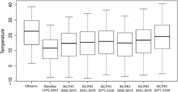
Figure 8. Box-and-whisker plots of maximum temperature for the period of observed and baseline (1976–2005), and future (2006–2035, 2041–2070, 2071–2100) from CCAM with RCP4.5 and RCP8.5.
Download figure:
Standard image High-resolution image
Figure 9. Box-and-whisker plots of precipitation for the period of observed and baseline (1976–2005) and future (2006–2035, 2041–2070, 2071–2100) from CCAM with RCP4.5 and RCP8.5.
Download figure:
Standard image High-resolution image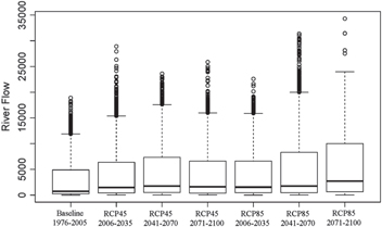
Figure 10. Box-and-whisker plots of river flow for the period of baseline (1976–2005) and future (2006–2035, 2041–2070, 2071–2100) from CCAM with RCP4.5 and RCP8.5.
Download figure:
Standard image High-resolution image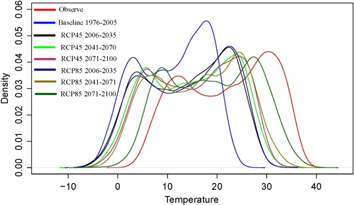
Figure 11. Probability density functions of daily maximum temperature for the period of observed and baseline (1976–2005) and future (2006–2035, 2041–2070, 2071–2100) from CCAM with RCP4.5 and RCP8.5.
Download figure:
Standard image High-resolution image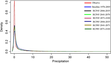
Figure 12. Probability density functions of daily precipitation for the period of observed and baseline (1976–2005) and future (2006–2035, 2041–2070, 2071–2100) from CCAM with RCP4.5 and RCP8.5.
Download figure:
Standard image High-resolution image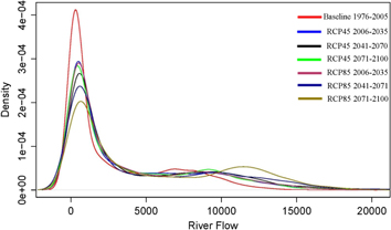
Figure 13. Probability density functions of Daily River flow for the period of baseline (1976–2005) and future (2006–2035, 2041–2070, 2071–2100) from CCAM with the RCP4.5 and RCP8.5.
Download figure:
Standard image High-resolution image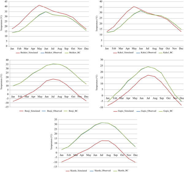
Figure 14. Mean monthly Climate Change and Bias Correction (using BES) for maximum temperature model simulated (red color), observed (blue color overlapping over green) and bias corrected (green color) for the period of 1976–2005 over selected stations mentioned in each graph of the UIB. Note: Similar graphical representation for minimum temperature of CCAM and RegCM (not shown here).
Download figure:
Standard image High-resolution image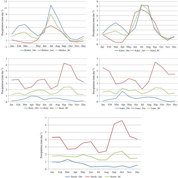
Figure 15. Mean monthly Climate Change and Bias Correction (using BES) for precipitation model simulated (red color), observed (blue color) and bias corrected (green color) for the period of 1976–2005 over selected stations mentioned in each graph of the UIB.
Download figure:
Standard image High-resolution image
Figure 16. Mean monthly Climate Change and Bias Correction (using MMCF) for precipitation model simulated (red color), observed (blue color overlapping over green) and bias corrected (green color) for the period of 1976–2005 over selected stations mentioned in each graph of the UIB. Note: Similar graphical representation for precipitation of RegCM (not shown here).
Download figure:
Standard image High-resolution image
Table 7. The average values of maximum temperature, minimum temperature, precipitation and river flow for the observed time period, baseline period (1960–1990) and future periods ((2006–2035, 2041–2070, 2071–2100), their corresponding errors are also presented. The observed river flow is not mentioned because the data on observed river flow is missing for some years.
| Duration | Max temperature | Min temperature | Precipitation | River flow |
|---|---|---|---|---|
| Observation | 21.50 ± 0.17 | 9.02 ± 0.14 | 1.95 ± 0.08 | — |
| 1976–2005 | 10.90 ± 0.13 | 0.69 ± 0.14 | 3.29 ± 0.10 | 2769 ± 64 |
| RCP4.5 | ||||
| 2006–2035 | 13.86 ± 0.15 | 1.54 ± 0.15 | 3.68 ± 0.15 | 3701 ± 80 |
| 2041–2070 | 14.89 ± 0.16 | 2.52 ± 0.14 | 3.77 ± 0.15 | 4066 ± 85 |
| 2071–2100 | 15.42 ± 0.16 | 3.07 ± 0.14 | 3.73 ± 0.15 | 3749 ± 81 |
| RCP8.5 | ||||
| 2006–2035 | 14.05 ± 0.16 | 1.67 ± 0.14 | 3.66 ± 0.14 | 3729 ± 79 |
| 2041–2070 | 16.12 ± 0.16 | 3.83 ± 0.14 | 3.78 ± 0.15 | 4532 ± 98 |
| 2071–2100 | 18.99 ± 0.16 | 6.51 ± 0.13 | 3.95 ± 0.16 | 5176 ± 97 |
Table 8. Stations used in the study at UIB, Pakistan.
| S. No | Station Name | Latitude | Longitude | Elevation |
|---|---|---|---|---|
| 1 | Kakul | 34 ° 11 ' | 73 ° 15 ' | 1308 . 0 meter |
| GariDupatta | 34° 13' | 73° 37' | 813.5 meter | |
| 2 | BalaKot | 34° 33' | 72° 21' | 995.4 meter |
| 3 | Gupis | 36° 10' | 73° 24' | 2156.0 meter |
| 4 | Bunji | 35 ° 40 ' | 74 ° 38 ' | 1372 . 0 meter |
| Gilgit | 35 ° 55 ' | 74 ° 20 ' | 1460 . 0 meter | |
| 5 | Astore | 35 ° 20 ' | 74 ° 54 ' | 2168 . 0 meter |
| Skardu | 35 ° 18 ' | 75 ° 41 ' | 2317 . 0 meter |
Note: The stations set in italic bold text are averaged into a single station to fulfill the five station limitation of the UBC model.
5. Summary and conclusion
The above projections of climate change and its impacts are a challenge for the mountainous UIB, which is influenced by snow and glacier melting. The CCAM model results indicate that future temperature is projected to increase. RCP8.5 shows more increase than RCP4.5 due to the high emission in RCP8.5. The temperature increase is relatively slower in the last half of the future century as compared with first half decade of the century in RCP4.5. The precipitation increase in both scenarios is almost the same while in 2071–2100 the precipitation increase is 12% (decreasing trend in comparison with 2041–2070) in RCP4.5 and 20% in RCP8.5 by 2071–2100. The results of RegCM model also indicate that the temperature and precipitation is increasing for the future periods. Significant biases were also observed between the simulation (for both temperature and precipitation) and observed data for the baseline period (1976–2005). Both the CCAM and RegCM model underestimate the temperature, whereas they overestimate the precipitation over UIB. However, the increasing trend of precipitation is uneven in contrast to temperature over UIB. To overcome these biases in the simulated data, statistical bias correction techniques were used. The same bias correction rules of base period were then applied to the future projections of model simulated data. After bias correction, the model data showed realistic results of monthly variation and climatology in the region that were in agreement with the spatiotemporal change of the observed precipitation and temperature. A similar process for bias correction is also applied for RegCM data. The UBC model was calibrated and validated for the simulation for future hydrological projection. The efficiency of the model was calculated using Nash-Sutcliffe statistics and the determination coefficient is 0.90 for our study region, which is considered as efficient for the hydrological model calibration (Berenguer et al 2005). The calibrated UBC model was then applied for the future river flow's projection for the period of 1976–2005, 2006–2035, 2041–2070, and 2071–2100 for CCAM and 2041–2050, 2071–2080 for RegCM.
The results of future river flow projections show an increasing river flow for all future periods as compared to the baseline time period (1976–2005) for CCAM. The highest river flow appeared during summer and this may possibly be due to the high increase in temperature that increases the melting of snow in summer. The results of river flow show an increasing trend during time periods 2006–2035 and 2041–2070. Meanwhile, the increasing trend during time period 2071–2100 is relatively low, even decreasing in RCP4.5 because the temperature precipitation increase is also slow in the same period in RCP4.5. The results of future river flow projections from RegCM input data also show increasing river flow for the period of 2041–2050 and 2071–2080. The results of river flow show an increasing trend during time period 2041–2050 (36%). Meanwhile, the increasing trend during time period 2071–2080 (56%) is relatively low.
The possible reason of increasing trend in river flow during the first half of the century may be the faster snow melting due to the increasing trend in temperature. In the last half of the century in RCP4.5, since the temperature and precipitation is not increasing with same trend as first half, the contribution to the river flow is lower. Our results correspond to the IPCC report (IPCC 2007), which states that temperature and precipitation are likely to increase along with river flow in this region and this might create more flooding in the first half of the century. A comparison of the results of RegCM and CCAM for the twenty first century shows that they are in agreement (increase in temperature, precipitation and river flow) to each other, and there is a smaller difference.
It is, therefore, concluded that both models (CCAM and RegCM) show increase an in temperature and precipitation over the UIB during the twenty first century, which provides the evidence that climate change is occurring in the region. These changes have the potential of melting snow in the UIB at a high rate with time and this could lead to a high river flow, which may affect the UIB due to the absence of any controlling reservoir (dam) and a limited flood management system. The forecasting ability in the lower areas downstream Tarbela reservoir is comparatively good and it has the capacity to control the flood water. In this study, the rivers of the Upper Indus may experience almost double river flow in 2041–2071 and the highest mean river flow (8913 cumecs in 2006–2035, 12 192 cumecs in 2041–2070 and 12 492 cumecs for 2071–2100) occurs in July, which is less than the observed river flow of 2010 super flood, but our results show a consistent increase in Jun-Aug. If there is any heavy rainfall event with this increased river flow, then it may exacerbate flash flood risk in the future, which will directly affect the hydrological dynamics and water resources of the region. However, the result (more water) of our study is a positive sign for agriculture food production, such as wheat, maize and rice, which are based on water availability from the irrigation system (Malik et al 2012). In order to reduce the risk of flood, new reservoirs need to be built to lower the effects of flooding and to address the protection of standing crops, natural resources, life losses, as well as to preserve the water for irrigation. A probabilistic approach is useful to understand the uncertainty associated with future climatic and hydrological projections. Predicting future river flows with uncertainties analyses needs more climate or hydrological models to ensemble enough results to be interpreted.
Acknowledgments
We thank Erika Coppola and Graziano Giuliani from ICTP, Michael Quick from the University of British Columbia, Canada, and Michelle van Vliet from IIASA for providing us with climatic data, models and valuable suggestions for this work. This study is supported by the National Basic Research Program of China (grant no. 2010CB428502, 2011CB952003), the Knowledge Innovation Program of the Chinese Academy of Sciences (KZCX2-EW-QN208), the project of National Natural Science Foundation of China (grant no. 41275082), and the R&D Special Fund for Public Welfare Industry (meteorology) by the Ministry of Finance and the Ministry of Science and Technology (GYHY201006014-04).