


Abstract
A solid-state single-photon source emitting indistinguishable photons on-demand is an essential component of linear optics quantum computing schemes. However, the emitter will inevitably interact with the solid-state environment causing decoherence and loss of indistinguishability. In this paper, we present a comprehensive theoretical treatment of the influence of phonon scattering on the coherence properties of single photons emitted from semiconductor quantum dots. We model decoherence using a full microscopic theory and compare with standard Markovian approximations employing Lindblad-type relaxation terms. Significant differences between the two approaches are found.
Export citation and abstract BibTeX RIS

Content from this work may be used under the terms of the Creative Commons Attribution 3.0 licence. Any further distribution of this work must maintain attribution to the author(s) and the title of the work, journal citation and DOI.
1. Introduction
Recent years have witnessed increased research interest in various quantum computing schemes and quantum information technologies [1, 2]. The central entity enabling quantum computers to perform certain types of computations many orders of magnitude faster than classical computers is the qubit. In the context of quantum optics, the quantum computing scheme proposed in [3] has attracted particular attention, as it only requires single-photon sources (SPS) and detectors as well as standard linear optical components, such as beam splitters and phase shifters. However, a requirement is that the single photons produced by the SPS need to be quantum mechanically indistinguishable. This places strict requirements on the SPS since any form of decoherence will inevitably make the single photons distinguishable from each other and hence unsuitable for quantum computations. While highly coherent single photons can be generated in atomic cavity QED settings, a solid-state platform appears more realistic for a practical SPS. However, in the solid state the quantum system is inherently coupled to its environment, leading to more decoherence channels and hence, in general, a smaller degree of indistinguishability.
In the low temperature and weak excitation regime, where a solid-state semiconductor SPS is expected to operate, the main source of decoherence stems from the interaction with phonons [4–6], in accordance with the limited number of experimental studies that have been performed [7–9]. Despite this, the vast majority of theoretical studies of indistinguishability have employed a simple Markovian pure dephasing rate description of the phonon-induced dephasing [10–17] or phenomenological descriptions of finite-memory dephasing processes [18], and only very recently have microscopic treatments been presented that explicitly take into account the cavity QED setting [19, 20]. The effect of phonons on the two-photon interference visibility has been investigated earlier [21], but without taking into account an optical cavity and considering a flat radiative reservoir.
The generation of indistinguishable single photons using continuous optical or electrical excitation [22–25] and pulsed electrical [26, 27] excitation has been demonstrated. A relatively high two-photon interference visibility was achieved in electrically driven SPSs [27], despite the system being incoherently pumped and the absence of cavity QED effects in the experiment. However, this high visibility was obtained using postselection which deteriorates the SPS efficiency.
Besides the study of indistinguishability, the importance of phonons in solid-state cavity QED has been well documented in recent years. Phonons have been found to be important in relation to emission spectra [28–30], spectral asymmetries in quantum dot (QD) lifetimes [31–33], and more recently, in describing Mollow triplets in coherently driven cQED systems [34–36].
1.1. Figures of merit
An SPS has several important figures of merit, namely the degree of indistinguishability, the emission efficiency into the desired mode, usually denoted as the β-factor, and the total collection efficiency. Here we consider only the first two; see [37] for an account of the total collection efficiency.
The degree of indistinguishability is measured in a two-photon interference experiment, first performed by Hong, Ou and Mandel (HOM) [38], which is illustrated in figure 1 (left). Here, two single-photon wavepackets are interfered on a 50/50 beam splitter, and in the case of completely indistinguishable photons, the two photons coalesce and exit through the same beam splitter output. Thus, there are no simultaneous 'clicks' in the detectors monitoring the two output arms, i.e. no coincidence events. However, even the smallest amount of decoherence will lead to changes between subsequently emitted photons, which thus become distinguishable and will lead to coincidence events. In figure 1 (right) we show a simulated result of typical HOM experiments, where the number of detector events is recorded as a function of the difference time τ = t1 − t2 between detector events in the output arms. The events clustered near τ = 0 appear due to the presence of pure dephasing and would be absent in the case of lifetime-limited single photons [39]. The other peaks, not centered around τ = 0, arise due to detector events between single photons separated by the repetition time, Trep, of the laser used to excite the emitter, and thus represent uncorrelated events. We define the degree of distinguishability as the normalized number of coincidence events [11], corresponding to taking the area under the structure at τ = 0 (shaded red in the figure) and dividing by the area of an unsuppressed peak (shaded green). Subtracting this number from unity, we obtain the degree of indistinguishability, formally expressed as [11]


where G(2)HOM(t + τ,t) is the second-order correlation function for the HOM experiment, G(2)uncorr(t + τ,t) yields the uncorrelated coincidence events, the green curve in figure 1 (right), and can be modeled as a HOM experiment without beam splitter, and the operator A is chosen corresponding to the relevant photon quantum field.

Figure 1. (Left) Illustration of the Hong–Ou–Mandel experiment, where single photons emitted from two cQED systems are interfered on a beam splitter and subsequent detector events are recorded. (Right) Simulated results of a HOM experiment with detector events as a function of the difference time τ = t1 − t2.
Download figure:
Standard imageAnother important figure of merit is the β-factor, describing the fraction of light emitted into the desired mode, which is most often the cavity mode due to its strong spatial directionality. We define the β-factor for a decay channel i of level j as

where

is the energy lost from level j due to the decay channel i, with γi,j being the corresponding decay rate, and nj(t) the occupation of the decaying level.
We note that this definition of the β-factor generalizes the commonly used expression involving exponential decay rates [40], which only holds in the weak light–matter coupling regime. Equation (3) can be employed in both the weak and strong light–matter coupling regimes and can furthermore include non-radiative decay channels, which becomes relevant whenever the quantum efficiency is significantly below unity.
In this paper we investigate the influence of phonon-induced decoherence on the degree of indistinguishability and efficiency of a semiconductor SPS. We treat phonon interaction both on a phenomenological level, through the inclusion of a pure dephasing rate using the Lindblad formalism, as well as using a full microscopic model including non-Markovian effects in the short-time limit [19]. We present novel results on the dependence of the indistinguishability on important parameters of the cavity QED system and review relevant results from the literature.
2. Theoretical model
To model the semiconductor SPS, we employ the standard Jaynes–Cummings model, including only the one-photon manifold. We neglect higher order manifolds and have explicitly tested this approximation by including the two-photon manifold, where numerically identical results were obtained, even in the regime of strong QD–cavity coupling. We expect that the pumping or driving terms need to be included before higher order manifolds become important [35, 41, 42]. The Jaynes–Cummings mode is parameterized by the QD–cavity coupling strength g and the QD–cavity detuning Δ = ωQD − ωcav. We include decay of the population of the excited QD state by a rate Γ, representing non-radiative processes and decay into leaky modes, but not the cavity, escape of cavity photons by a rate κ, and we allow for pure dephasing with a rate γ of transitions connected to the excited QD level |e〉. Furthermore, we include an additional excited state in the QD, called the pump level and denoted as |p〉, from which an excitation may relax into the excited QD state by a rate α, e.g. due to phonon scattering [43]. This simulates non-resonant excitation of the QD, which is often employed experimentally and is known to affect the indistinguishability [11, 12, 14] by introducing the so-called time jitter into the system. In figure 2 (left) a schematic illustration of the total system is presented, while figure 2 (right) shows a few typical cavity designs.

Figure 2. (Left) Schematic illustration of the Jaynes–Cummings model including an additional pump level. The rates α, Γ and κ represent transitions between the indicated levels, while γ is the rate of pure dephasing associated with the level e. Finally, g is QD–cavity coupling strength and Δ = ωe − ωg − ωcav = ωQD − ωcav is the QD–cavity detuning. (Right) Illustrations of a micropillar cavity and a photonic crystal cavity with an embedded QD (red triangle).
Download figure:
Standard imageThe coherent processes are modeled by the Hamiltonian

where ℏωp, ℏωe and ℏωg are the QD state energies, ℏωcav is the cavity photon energy, ℏg is the QD–cavity coupling, σij = |i〉〈j| are QD operators, and a and a† are cavity photon operators. We simulate the dynamics using the reduced density matrix formalism [44, 45], obeying the equation of motion (EOM)

where loss is included through Lindblad operators of the form

To simplify the dynamical equations, we move to a rotating frame defined by the following operator:

Operators transform according to O → T†(t)OT(t). The transformed Hamiltonian equals the well-known Jaynes–Cummings Hamiltonian

where Δ = ωe − ωg − ωcav = ωQD − ωcav is the QD–cavity detuning.
While the reduced density matrix provides access to all one-time expectation values of the cQED system, two-time correlation functions are needed to calculate the degree of indistinguishability (equation (2)). These are obtained using the quantum regression theorem (QRT) [45], which holds for Markovian reservoirs.
3. Markovian decoherence: pure dephasing and time jitter
In this section we investigate the influence of phenomenological Markovian sources of decoherence on the degree of indistinguishability. These effects can be modeled with a phenomenological pure dephasing rate within the Lindblad formalism and can dominate the decoherence in the system, especially in the cases where phonons are suppressed, e.g. in phononic band-gap materials [46] or in thin wire structures. Also we consider the effect of time jitter that arise when the system is excited non-resonantly.
3.1. Weak quantum dot (QD)–cavity coupling
We start by considering the simplest physical scenario, namely the limit in which the cavity can be adiabatically eliminated from the equations and thus effectively acts as an additional loss channel for the QD. Formally, the elimination is performed by integrating out the photon-assisted polarizations, given by 〈aσeg〉(t) and 〈a†σge〉(t), and performing the Markovian long-time limit in the resulting memory integrals. In order for the adiabatic elimination to be valid, the QD–cavity coupling must be significantly smaller than the total decoherence rate or the QD–cavity detuning (or both), formally: g ≪ γ + (Γ + κ)/2, Δ. Performing the elimination results in an additional irreversible decay rate associated with the QD into the cavity [47], given by the Purcell enhanced rate

where γtot is the total decoherence or dephasing rate. This significantly simplifies the dynamical equations, with the new governing equation taking the form

where

According to equation (2), the degree of indistinguishability of photons emitted from the QD may be obtained by determining 〈σee(t)〉 and 〈σeg(t + τ)σge(t)〉. These functions are readily obtained from equation (11)

and

assuming that the electron was initially in state p of the QD. From equation (1) we then get the degree of indistinguishability of photons emitted from the QD

This approximate analytical expression includes both the effect of pure dephasing and the influence of time jitter. While analytical expressions have been presented earlier, these have been limiting cases of equation (15), either neglecting time jitter [10] or neglecting pure dephasing [14].
The β-factor of the SPS may be easily obtained in the adiabatic regime, as analytical expressions are available for both the QD and cavity populations. To facilitate this we express the QD background rate as Γ = Γrad-bg + Γnon-rad, where Γrad-bg is the radiative background rate in the absence of the cavity, and Γnon-rad represents non-radiative decay channels. In the adiabatic regime, the cavity population obeys the following equation: ∂tncav(t) = −κncav(t) + RnQD(t) ≈ 0, and hence the cavity population is determined by the QD population as

Using this relation the total number of photons emitted from the cavity decay channel becomes

while the energy not lost through the cavity is


where we used equation (4). The β-factor for the cavity then simply becomes


where we introduced the Purcell factor as FP = R/Γbulk and where Γbulk is the radiative decay rate in a bulk medium. In the situations where non-radiative decay is negligible, the last term in the denominator may be safely omitted [40].
Due to the simple analytical form of the expressions derived for the indistinguishability of photons emitted from the QD, equation (15), and the cavity β-factor, equation (20), considerable insight into the physics can be obtained by simple inspection.
The β-factor is only governed by two quantities, namely the Purcell factor and the background QD rate Γ. To efficiently collect the light emitted from the QD–cavity system, it is preferential to have it emitted into the cavity mode, featuring a well-defined far field emission pattern that may be highly directed toward the collection optics [37]. The cavity β-factor should therefore be as close to unity as possible, as obtained either by increasing the Purcell factor, via the Purcell rate R, equation (10), or by decreasing the QD background decay rate Γ via the suppression of leaky/radiation modes and non-radiative decay.
The expression for the indistinguishability, equation (15), has two factors, namely Γeff/(Γeff + 2γ) and α/(α + Γeff). The first factor arises due to the presence of pure dephasing in the system, leading to decoherence of the QD and thus loss of indistinguishability of the single photons emitted from the system. Decoherence due to pure dephasing can be combated by increasing the effective decay rate of the QD Γeff, which is typically achieved by exploiting the Purcell effect [7, 8]. The second factor arises as the QD is assumed to be initialized in the pump level |p〉, where it needs to relax to the excited level |e〉 before it can emit the photon. While the relaxation process from the pump to the excited level does not by itself introduce decoherence of the QD–cavity system, it introduces uncertainty in the emission time of the photon from the QD. This translates into a non-ideal temporal overlap of the two interfering photons on the beam splitter in the HOM experiment, inevitably leading to a lower degree of two-photon interference. Due to the nature of this process, it is often referred to as time jitter [11, 14, 17]. The detrimental effect of time jitter is minimized by decreasing the effective QD decay rate or increasing the decay rate from the pump to the excited level α.
From the analysis above, it is clear that maximizing the indistinguishability by simultaneously combating time jitter and pure dephasing by changing the effective QD decay rate cannot be achieved. This is illustrated in figure 3 where we show the indistinguishability and β-factor for the cavity as a function of the QD–cavity coupling g, for realistic parameters representative of the weak coupling (WC) regime. For the β-factor, a monotonic increase is observed, since increasing the QD–cavity coupling g rapidly increases the Purcell factor, according to the scaling FP∝g2. The indistinguishability is also seen to increase initially with the QD–cavity coupling, but eventually starts decreasing again. This behavior is easily understood as referring to the discussion above of the analytical expression. The initial increase is caused by the QD decaying faster for a larger coupling rate, thereby leaving the pure dephasing processes a smaller time span to decohere the system. For some value of g, however, the decay of the QD has become so fast that it is comparable with the relaxation rate from the pump level and the effect of time jitter starts reducing the indistinguishability. Physically, a faster QD decay results in shorter temporal photon wavepackets and hence a stronger effect of the uncertainty in the arrival time on the beam splitter. For the curves where the relaxation rate α tends to infinity, the indistinguishability continues to increase as a function of g, as expected when no time jitter is present. Increasing the pure dephasing rate is seen to only weakly affect the β-factor, while it causes a significant lowering of the indistinguishability for all values of g.

Figure 3. Indistinguishability (red, blue, and green lines, from equation (15)) and cavity β-factor (black lines, from equation (20)). (Left) Parameters: ℏκ = 150 μeV (solid), 300 μeV (dashed). ℏα = 10 μeV (red), 50 μeV (blue) and ∞ μeV (green). Other parameters: ℏγ = 1 μeV, ℏΓ = 1 μeV, and ℏΔ = 0 μeV. (Right) As in (left) except that ℏγ = 5 μeV.
Download figure:
Standard imagePure dephasing and time jitter have both been shown to negatively influence the degree of indistinguishability. Despite their common detrimental effect, these two mechanisms are, in fact, of fundamentally different nature. Pure dephasing thus arises due to phase destroying processes, whereas time jitter comes about through population decay. While pure dephasing is intrinsic to the system, time jitter can be reduced by employing quasi-resonant excitation or eliminated using resonant excitation. Indeed, resonant optical excitation of a single QD has been demonstrated experimentally in weak laser-guiding cavities [48] as well as in conventional cavities employed in semiconductor cQED [49–51], leading to the complete vanishing of time-jitter effects. For this reason we will, in the following, neglect the effect of time jitter and concentrate on decoherence induced by the more fundamental pure dephasing processes.
For completeness, we will briefly discuss the modeling of indistinguishability in atomic cavity QED. In a typical atomic setting, reservoirs couple weakly to the system of interest and do not display significant structure in the spectral domain, for which reason such reservoirs are well described by the memory-less Markovian Lindblad formalism used above. Furthermore, often only the regime of weak light–matter coupling is relevant and hence the single-photon temporal waveform can be assumed to be exponential. Therefore, theories aimed at atomic cavity QED [15, 52] are formulated in terms of assumed known wavefunctions for single-photon wavepackets and the effect of pure dephasing is incorporated using assumed known probability distributions of the single-photon center frequency. While this approach is simple to deal with and in some cases can give analytical results, it suffers from not taking into account the microscopic origin of the emission processes and the decoherence processes, which generally cannot be treated separately. We will treat such an example below in section 4 where the light–matter system is in the strong coupling regime, which has direct consequences for the phonon-induced decoherence.
3.2. Strong QD–cavity coupling
In the previous section the adiabatic elimination of the photonic degrees of freedom was seen to result in an analytically solvable system, leading to physically intuitive expressions for the indistinguishability and β-factor. For the more general case where the cavity cannot be eliminated, we have to resort to a numerical solution of the governing EOMs. This enables us to investigate both the intermediate and strong coupling regimes between the QD and cavity, both of which are accessible in present-day samples [9, 53]. For these simulations we employ the full model presented in section 2, with the exception of omitting the pump level |p〉 and instead initiating the system in the excited state |e〉 of the QD. We calculate the indistinguishability for photons emitted both from the QD, through 〈σeg(t + τ)σge(t)〉, and from the cavity, through 〈a†(t + τ)a(t)〉.
The results of the simulations are shown in figure 4 as a function of the QD–cavity coupling g, where for comparison we included the corresponding quantities obtained using the analytical expressions from section 3.1. The parameters have been chosen so that the lowest values of g correspond to the WC regime and the largest correspond to a system well into the strong coupling regime, see the figure caption for details.

Figure 4. Indistinguishability and β-factor comparison for QD and cavity using analytical expressions (an.) from equations (15) and (20) and full numerical solution (num.). Parameters: ℏκ = 100 μeV, ℏγ = 1 μeV, ℏΓ = 1 μeV and ℏΔ = 0.
Download figure:
Standard imageAs expected from the discussion in the previous section, the analytical expressions predict an ever increasing degree of indistinguishability and efficiency as the QD–cavity coupling is increased, eventually approaching unity. For the numerical results we observe a behavior for small g values that closely follows the analytical results; however, close to ℏg ≈ 25 μeV the two models start to deviate significantly, indicating the break-down of the adiabatic elimination procedure that was employed to arrive at the analytical results. Instead of approaching unity, the numerical results settle at values significantly below unity for both the indistinguishability and β-factor.
The physical reason for the initial increase of the indistinguishability and of the efficiency with g-value is an increase of the Purcell effect as the QD–cavity coupling is increased, while the saturation of these quantities arises due to a clamping of the effective decay rate of the QD. The clamping occurs as the system enters the strong coupling regime, where the effective QD decay rate becomes independent of g [54, 55].
4. Non-Markovian decoherence: coupling to longitudinal acoustical phonons
It has recently been demonstrated that in order to properly describe the decay [31, 33, 56] and the emission spectra [30, 34, 35] of a QD in a cavity, it is necessary to include phonons and in some cases even the structure of the phonon reservoir. The interaction between a small system and a structured reservoir is known to give rise to memory or non-Markovian effects in the short-time limit, which in the case of a semiconductor QD coupled to longitudinal acoustical (LA) phonons typically implies the first 5 ps of the time evolution [56].
In the studies referred to above, the long-time Markovian limit has been taken, meaning that the structured phonon reservoir is probed at specific frequencies. This should be contrasted with the phenomenological Lindblad theory, which typically assumes a spectrally structure-less, and thus memory-less, reservoir in which the Markovian long-time limit becomes exact. The Lindblad procedure results in constant scattering rates, whereas in the long-time Markovian limit the rates become energy dependent due to the structure of the reservoir.
The distinction between the Lindblad theory and the long-time limit of a structured reservoir becomes especially important if the reservoir spectrum has significant variations across the spectral bandwidth of the cQED system, e.g. the vacuum Rabi splitting, which is often the case in state-of-the-art cQED systems. In this case the mathematical structure of the long-time Markovian and Lindblad theories is different and produces both quantitative and qualitative results. We note that the long-time Markovian theory may be brought into a Lindblad form under the secular approximation [44, 57].
The long-time Markovian limit should be contrasted with the short-time non-Markovian limit, where all phonon frequencies are sampled through virtual processes. Reasonably good agreement between theory and experiment has been established in all of the studies referred to above, indicating that the long-time Markovian limit constitutes a good approximation in these situations. For the decay dynamics this is easily understood since the QD population only experiences the short-time regime for approximately 5 ps, whereas typically QD lifetimes are of the order of several tens to hundreds of ps even when the decay is enhanced by the Purcell effect. Hence short-time non-Markovian effects appear to be negligible for the decay dynamics.
If we want to investigate the effect of a non-Markovian phonon reservoir on the indistinguishability, the situation is fundamentally different, since the indistinguishability is derived from a two-time function, 〈A†(t + τ)A(t)〉, as opposed to a population, which is derived from a one-time function, 〈A†(t)A(t)〉. The correlation function 〈A†(t + τ)A(t)〉 continuously (at each instant t) probes events separated temporally by τ through the operators A and A†, and consequently the indistinguishability is expected to be much more sensitive to short-time non-Markovian or memory effects. The continuous probing means that short-time non-Markovian effects are important during the entire lifetime of the QD excitation and not just during the initial 5 ps.
In the previous section we used the QRT to calculate 〈A†(t + τ)A(t)〉, which was possible as we limited our attention to Markovian reservoirs included through the Lindblad formalism. If we include phonons in a non-Markovian reservoir description like, e.g., the time convolution-less approach [32, 58], the QRT can no longer be rigorously employed as it only holds for memory-less reservoirs. Several non-Markovian extensions to the QRT exist [59–64], but all of them significantly complicate the calculation of two-time functions as compared to the simple QRT procedure. For this reason we include the phonons directly in the QD–cavity system, rather than as a reservoir, thereby treating them on an equal footing as photons and electrons. This enables us to still employ the QRT and retain all non-Markovian effects arising from the phonon interaction in the calculated two-time functions. This kind of exact diagonalization (ED) approach is usually not feasible due to the very large dimensionality of the phonon Hilbert space, but by following a procedure to be described below, the problem becomes numerically tractable.
4.1. The Jaynes–Cummings model including effective phonon modes
In this section we will describe the enabling step, due to Hohenester [65], for performing the ED procedure consisting of replacing the original set of three-dimensional (3D) phonon modes with an effective set of one-dimensional (1D) modes and employing an efficient cut-off scheme. The reduction in dimensionality is necessary as a full treatment of 3D phonon modes would be beyond the computational capabilities of most university clusters, whereas a 1D model can be solved even on a personal laptop.
Our starting point for deriving the effective 1D modes is the Hamiltonian for the Jaynes–Cummings model including the coupling to LA phonons, see [56] for details, describing the unitarily coupled electron–photon–phonon system

HJC is defined in equation (9), Mk is the QD-phonon matrix element, ωk is the phonon dispersion relation and b†k, bk are bosonic phonon operators. The phonon wavevector k = (kx,ky,kz) is a 3D vector which we would like to reduce to an effective 1D vector. To this end, we note that our model describing the LA phonons is assumed to be isotropic; hence no single direction in space is preferred by these modes, rendering the phonon dispersion relation a function of the length of k alone, ωk = f(|k|) ≡ f(k). The phonon matrix element, however, depends explicitly on the electronic wavefunctions ϕν(r) as

where d is the material density, cs is the speed of sound, V is the quantization volume and Dν is the deformation potential, see [56] for the numerical values. If we employ an isotropic harmonic confinement, we obtain spherically symmetric wavefunctions given by

Inserting this into the phonon matrix element, we obtain

which only depends on k. We have now reduced all numerical quantities in the Hamiltonian to depend only on k; hence every phonon process will take place on spherical shells in k-space with a radius of k.
To obtain an effective description of this physical situation, we consider the phonon reservoir correlation function, see, e.g., [32], which plays an essential role in most reservoir theories. For simplicity we evaluated it at zero temperature, and take the integral limit of the sum


where we introduced the effective phonon matrix element

This shows that one may obtain an arbitrarily good approximation to the correlation function D>(t) by replacing the original 3D modes with an effective discrete 1D set with a slightly modified matrix element  and discrete (radial) wavevectors kp. Motivated by this, we replace the original Hamiltonian by

where ωp ≡ ωkp = cskp and  are standard bosonic operators for the new effective phonon modes. An effective phonon Hilbert space can now be constructed using phonon Fock states of the form

where the following weight function is determined for each state:

and only states where Λ >  cut-off are included and αmax is the largest dimensionless coupling strength. This leads to the systematic inclusion of the most important states, as illustrated in figure 5(a), where the phonon Hilbert space is presented graphically with each value on the second axis representing a specific phonon state |n0,n1,...,nN−1〉 with colors indicating the number of excitations in the given mode. The figure has a clear structure separating the one-phonon (bottom), two-phonon (middle) and three-phonon (top) manifolds. The shaded area shows the mode weight function αp, equation (31), and the right side shows the state weight function Λ({n}), equation (31), used for selecting the most important states. We emphasize that no uncontrolled approximations have been employed, we have merely restricted ourselves to consider spherical QD models, as is common in the literature [35, 66], and employed a controlled truncation of the phonon Hilbert space. This renders the approach numerically exact, assuming it will fit in one's computer system.

Figure 5. (a) Phonon Hilbert space including up to three phonon excitations for a set of illustrative parameters: cut-off = 4 × 10⁻³, Δk = 0.05 nm−1, where kp = Δk × p. Also included are the mode weight function αp, as the shaded region, and the phonon state weight function Λ({n}), equation (31). (b) Illustration of M, equation (36), in its original basis where blue (white) indicate non-zero (zero) values. (c) The same as (b) but represented in optimized basis revealing decoupled sub-blocks.
Download figure:
Standard imageWe formulate the equations of motion in terms of the transpose of the density matrix

Furthermore, we remap the problem onto a vector form using the vec operation, which is defined as the 'row-stacked' version of a matrix X

From this definition the following useful identity for a three-matrix product can be derived [67]:

which may be used to obtain

where the coupling matrix M is given by


where H is the Hamiltonian, (Γi,Oi) are Lindblad pairs and I is the identity matrix. In figure 5(b) we show the N2 × N2 matrix M, where N is the number of states in the total Hilbert space, which may easily reach values of several thousands in real simulations. Despite being quite sparse, M does not immediately seem to contain any structure that can simplify the ensuing numerics. From considerations of the coupling processes represented by the governing dynamical equation, however, we do expect M to contain more information than is needed to calculate relevant dynamical quantities, i.e. we expect M to contain decoupled subblocks. To reveal this structure, we employ graph theoretical methods for finding the connected components of a graph/matrix, which are freely available in the Python-based open source toolbox Scipy [68]. The result of this procedure is shown in figure 5(c), where the original basis states have been reordered to reveal several decoupled blocks along the diagonal of M. The subblock containing the relevant elements of the density matrix can now be employed in the numerics with significant reductions in both memory and cpu requirements.
We now proceed to solve the Master equation, employing the effective phonon modes in the unitary part of the equation as

while including standard Lindblad terms for the cavity and QD as above. This EOM is also used to calculate two-time correlation functions using the QRT, including all non-Markovian effects arising from the interaction with phonons. The phonon system is initiated in its vacuum state, corresponding to an initial temperature of T = 0 K, in which case no thermal phonons are excited. We expect this initial state to describe the fundamental limitations imposed by phonon interactions on the degree of indistinguishability. The method is not limited to zero temperature, but higher temperatures strongly increase the size of the phonon Hilbert space needed to ensure numerical convergence of the results. This was tested explicitly using finite-temperature analytical solutions to the so-called independent boson model [69]. To simulate an effective QD–cavity detuning of zero, we include a finite detuning of ℏΔ = ℏΔpol = 27.78 μeV to compensate for the phonon-induced polaron shift.
All results obtained using our ED approach will be compared with the standard pure dephasing rate description, discussed in previous sections, governed by the equation

where the pure dephasing γ is chosen to provide a reasonable fit to the ED result, to account for the effect of phonons.
4.2. Dependence on the QD–cavity coupling strength
In figure 6 we show the degree of indistinguishability for light emitted from the QD and cavity as a function of the QD–cavity coupling strength g. We include the results for the ED approach where up to two phonon excitations are present in the effective phonon modes. Sampling the three-phonon excitation manifold we estimate an error of at most 0.1% on the presented results. In the limit of small QD–cavity coupling strength ℏg ⩽ 20 μ eV, our ED approach suffers from long integration times. However, in this WC regime the cavity may be adiabatically eliminated, see section 3.1, and the phonons can be treated exactly [21, 62, 63]. The indistinguishability of photons emitted from the QD is then obtained as

where ![${\mathrm { Re}}[\varphi (\tau )]=\sum _{\mathbf {k}} |M^{\mathbf {k}}/(\hbar \omega _{\mathbf {k}})|^2\cos (\omega _{\mathbf {k}} \tau )$](https://content.cld.iop.org/journals/1367-2630/15/3/035027/revision1/nj453046ieqn3.gif) is the polaron correlation function at T = 0 K. A correspondingly simple expression for the cavity cannot be obtained. For comparison we include the result of the phenomenological Lindblad theory discussed above.
is the polaron correlation function at T = 0 K. A correspondingly simple expression for the cavity cannot be obtained. For comparison we include the result of the phenomenological Lindblad theory discussed above.
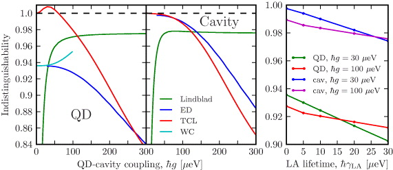
Figure 6. (Left) Calculated degree of indistinguishability for emission from the QD and cavity as a function of the QD–cavity coupling g. Results are included for the ED approach, along with the corresponding Lindblad results and the weak QD–cavity coupling (WC) results for the QD. (Right) Calculated degree of indistinguishability as a function of phonon decay rate. Parameters: ℏΓ = 1 μeV, ℏκ = 100 μeV, ℏΔ = 27.78 μeV, and ℏγ = 1 μeV.
Download figure:
Standard imageThe ED approach leads to results which are markedly different from the predictions of the simple Lindblad model, discussed in previous sections. Instead of an indistinguishability that increases with coupling strength, as predicted by the Lindblad theory, the ED approach leads to a decrease in indistinguishability, especially pronounced for large QD–cavity coupling. For small QD–cavity coupling, ℏg ⩽ 30 μeV, the indistinguishability for the QD depends only very weakly on g, and we expect a similar behavior for the cavity. The weak dependence on g can be understood from equation (40), as the effective decay time of the QD, Γ−1eff, needs to be comparable with the memory depth of the phonons, before the Purcell enhancement of Γ−1eff can significantly influence the indistinguishability. The memory depth is given by the decay time of Re[φ(τ)] being approximately 5 ps. It is interesting to note the divergence between the ED and WC results for ℏg ⩾ 30 μ eV, which occurs when back-action from the cavity starts to become important. In the Lindblad theory, a weak maximum occurs in the indistinguishability for the cavity emission; however, it only yields an indistinguishability which is 0.17% larger than the saturated value at large g.
The interaction with phonons is not the only source of decoherence for the emitted photons, and in situations where the phonon decoherence is either weak, e.g. in the limit of small QD–cavity coupling, or suppressed, e.g. through phononic band-gap effects [46], these additional sources may become significant. One such source is random nuclear field fluctuations, causing the energy levels in the QD to fluctuate giving rise to the pure dephasing effect. However, the corresponding rate is typically small and has been experimentally demonstrated [70] to be significantly smaller, ℏγfluc ≈ 0.07 μeV, than the pure dephasing rates employed here, which are typically ∼1 μeV. Another source is excess charge fluctuations in the spatial vicinity of the QD. These charges could be situated on the surfaces of the holes in the photonic crystal, the sides of a micropillar cavity, trapped in impurities inside the semiconductor bulk, or could reside in the wetting layer from above-band excitation. Coupling to charges in the wetting layer is known to strongly influence cavity QED properties [29], especially under detuned conditions; however, these effects can be avoided using quasi-resonant or resonant excitation of the QD. The influence of charges trapped on the outside of the structure or in impurities is very hard to estimate, as it depends both on the excitation mechanism, the specific system and its history. However, usually the influence can be reduced by employing high-quality samples and carefully designed experiments.
We start out by briefly explaining the basic physics of the ED results in the spectral domain [19] and afterwards we will present the corresponding analysis in the spatial domain. The main reason for the difference between the Lindblad and ED results is that while the Lindblad theory assumes a constant pure dephasing rate as a function of g, the microscopic treatment of the phonon interaction in the ED approach gives rise to a dependence of the phonon-induced dephasing processes on the QD–cavity coupling g. It turns out that the concept of an effective phonon density [56], defined below, is very useful in understanding the results

This function is closely related to the spectral function in reservoir theory, and gives the number of phonon modes at a given frequency available for scattering. For instance, it is directly related to recently observed spectral asymmetries in QD lifetimes [33]. For an example spectrum please see figure 7(a). Due to the coupling between the QD and cavity, these systems form a polaritonic quasi-particle with eigenenergies  for the upper (u) and lower (l) branches. An energy splitting of
  thus emerges, which is important in relation to the effective phonon density, as phonons may cause transition between these states.

Figure 7. (a) Effective phonon density, equation (41), at T = 0 K. (b), (c) Absolute value of the phonon displacement field, equation (42), as a function of time and distance from the QD center. (d), (e) Population dynamics for the QD and cavity. (f) Phonon displacement field as a function of time at a distance of 20 nm from the QD center. Parameters are as in figure 6.
Download figure:
Standard imageThe nearly constant value of the indistinguishability observed for small g, figure 6, reflects that the Purcell effect is weak and that the QD decays on a time scale that is much longer than the memory time of the phonon reservoir, as discussed above. In this regime, phonon-induced dephasing is dominated by virtual processes, where the entire effective phonon density is sampled. For increasing g the Purcell effect increases, leading to a faster decay of the QD and one would expect a higher degree of indistinguishability. However, the phonon dephasing also becomes stronger, since now the larger polariton splitting means that the effective phonon density can be sampled at larger frequencies, ω ≈ 2g, where the density is larger. The two effects compete, but the increasing Purcell effect is not able to counteract the increase of dephasing and the indistinguishability drops for both QD and cavity emission. This is merely a qualitative explanation, since the ED theory does not contain a phonon-induced dephasing rate, but rather the decoherence is governed by the many variables in the coupled QD–cavity–phonon system. As g increases further, the Purcell effect saturates as the system moves into the strong coupling regime, while the dephasing continues to increase, leading to the dramatic drop in indistinguishability.
For completeness we also include results for the indistinguishability calculated using the so-called time convolution-less (TCL) method [32, 44, 56, 58], which treats the phonon interaction microscopically, but only in the long-time Markovian limit where the virtual processes in the short-time regime are neglected. We note that the Markovian QRT was employed to calculate the relevant two-time functions [35, 66]. The TCL qualitatively captures the large drop in indistinguishability for large QD–cavity coupling; however, large quantitative deviations are observed, especially for the QD emission. Interestingly, the TCL even predicts unphysical above-unity values of the indistinguishability for the cavity emission, see the discussion in [44].
It is well known that anharmonic processes exist in which a high-energy phonon decays into two phonons of smaller energy, giving rise to a finite phonon lifetime. Furthermore, it has been shown that phenomenologically adding a finite lifetime to LA phonons coupled to a two-level QD yields a non-zero zero-phonon linewidth [71], corresponding to phonon modes being available at zero frequency. To investigate the influence of finite phonon lifetimes on the indistinguishability, we add Lindblad decay terms  to equation (38), causing all phonon modes to decay with a rate γLA. The results are shown in figure 6 (right) where the indistinguishability is shown for ℏg = 30 and 100 μeV as a function of γLA. The shortest lifetime is 22 ps which is significantly longer than the extent of the short-time non-Markovian regime. The results show that the degree of indistinguishability decreases for increasing phonon decay rate, as expected from previous studies on dephasing in QDs [71]. We also observe that the indistinguishability decreases faster for small QD–cavity coupling strengths than for large strengths. This is due to the fact that the finite phonon lifetime contributes with dephasing being independent of g [71], which acts as a background to the g-dependent dephasing discussed above. Hence for small g the background is relatively stronger compared to large g, where the g-dependent dephasing is large, and thus we observe a different slope as a function of g. Interestingly, we observe an intersection between the curves for small and large g, implying a qualitative shift in behavior from a monotonic decrease as a function of g as observed for γLA = 0, to a situation where the largest degree of indistinguishability is found at intermediate values of the QD–cavity coupling strength.
Rather than explaining the physics in the spectral domain, a more direct physical interpretation is possible by considering the real-space dynamics of the phonon field. This is done by calculating the displacement field of the phonons [72, 73]


In figures 7(b) and (c) we show the phonon displacement field for a small, ℏg = 30 μeV, and large, ℏg = 200 μeV, value of the QD–cavity coupling, while figures 7(d) and (e) display the corresponding population dynamics for the QD and the cavity.
For small QD–cavity coupling, we observe the emission of phonon wavepackets shortly after the initial excitation of the QD. The phonon emission occurs due to the very fast (assumed instantaneous) excitation of the QD, which 'shocks' the lattice and it reacts by emitting energy in the form of a phonon wavepacket [65]. After the initial emission, the dynamics in the QD occurs on a sufficiently slow timescale so that the lattice can adiabatically adjust to the time-varying QD excitation and no additional phonon emission events are observed. For large QD–cavity coupling, we also observe the initial emission of a phonon wavepacket; however, now the dynamics in the QD is no longer slow, due to the presence of fast Rabi oscillations, and the lattice is seen to be strongly displaced whenever the QD is in the excited state. As opposed to the previous case, the fast QD dynamics does not allow the lattice to follow adiabatically and smaller phonon wavepackets are emitted throughout the lifetime of the excitation. This is more clearly seen in figure 7(f), comparing the displacement field at a distance of 20 nm from the QD for the two cases, where for the small QD–cavity coupling only the initial wavepacket is seen, while for larger QD–cavity coupling subsequent wavepackets are also observed. The emission of phonon wavepackets leads to decoherence, as the emitted wavepacket encodes information on the quantum properties of the QD–cavity system, which is lost into the phonon reservoir. Hence the emission of more phonon wavepackets leads to a larger rate of decoherence.
For completeness we mention that several theoretical methods exist for treating few-level, and especially two-level, systems interacting with bosonic reservoirs such as phonons. Systematic many-body methods, such as the correlation expansion [74], have successfully been applied to the QD–phonon problem [66, 75, 76]; however, they often suffer from large numerical efforts, which tend to mask the underlying physics. Related to the TCL are polaron transformed versions [35, 56, 77–79], where phonons are included to high order through a unitary transformation, and also variational improvements [80]. Also, the effect of a semi-classical driving field has been investigated using the TCL [81]. Both these improvements to the TCL are essential in the regime of high temperatures and strong coupling strengths. Another class of methods are those based on path integrals. A review of path integrals especially focusing on two-level systems can be found in [82], and recently, efficient numerically exact algorithms were developed that are capable of treating a certain subclass of systems at arbitrary parameters [83–85].
4.3. Optimizing indistinguishability through cavity design
Whereas the Lindblad model for phonons suggests that indistinguishability is improved by maximizing the QD–cavity coupling strength, our ED approach predicts that the maximum indistinguishability is obtained at relatively small coupling strengths as illustrated in figure 6. In situations where phonons dominate the decoherence, an ideally engineered SPS should thus feature g and κ chosen in the parameter region of maximum indistinguishability according to figure 6.
An attractive system for engineering an SPS is the semiconductor micropillar cavity [86] illustrated schematically in the inset of figure 8. It features vertical emission combined with a Gaussian beam profile and it allows for independent control of the basic cQED parameters g and κ. They are related to the cavity Q factor as κ = ωcav/Q and to the optical mode volume Vmode as g = (πe2f/(4πr0 mVmode))1/2, where f is the oscillator strength, chosen as f = 10 in the following, m is the free-electron mass, r is the dielectric constant assumed to have the value 11.97 for GaAs, 0 is the vacuum permittivity and finally e is the electron charge.

Figure 8. (Left) Calculated QD–cavity coupling strength g for a QD in a micropillar as a function of pillar diameter. The inset shows a schematic illustration of a micropillar structure. (Right) Calculated cavity decay rate κ for a micropillar as a function of pillar diameter and for a varying number of top mirrors. The star indicates the diameter for which the maximum degree of indistinguishability in figure 6 is obtained.
Download figure:
Standard imageTo identify optimum geometrical parameters for realizing micropillar SPS of indistinguishable photons, we present in figure 8 calculations of g and κ as a function of pillar radius for a standard MP design based on a λ spacer in the GaAs/AlAs platform with a design wavelength of 950 nm. The design is identical to that in [87] and the QD is assumed to be positioned in the center of the nanowire. We vary the number of layer pairs Ntop in the top distributed Bragg reflector while keeping a fixed number Nbottom = 28 in the bottom mirror. The computations are performed using the eigenmode expansion technique [88] with improved perfectly matched layers [89].
While the QD–cavity coupling strength g is basically independent of Ntop in this parameter regime, figure 8 (left), the dependence of κ on pillar radius and Ntop is more complicated. In the large-radius regime, the pillar can be considered as a 1D system and κ is simply a function of Ntop. For shorter radii, variations in κ are observed. The origin of these variations is poor mode matching between the cavity and the distributed Bragg reflector (DBR) Bloch modes resulting in coupling to the propagating Bloch modes [90] in the DBR mirrors. This coupling can be suppressed by more advanced Bloch-wave engineered adiabatic cavities [91].
We can thus easily control g and κ in our design by choosing the pillar radius and Ntop according to figure 8. We observe that a pillar radius of 850 nm combined with a number of top layer pairs Ntop = 17 keeps us in the region of maximum indistinguishability presented in figure 6. Furthermore, this choice yields an efficient SPS, as it maximizes the β-factor by selecting the largest possible QD–cavity coupling g, without sacrificing the indistinguishability of the emitted photons.
5. Conclusion
In this paper we have presented a comprehensive theory of single-photon indistinguishability in semiconductor cQED. In the first part, we modeled the decoherence processes using phenomenological Markovian Lindblad pure dephasing terms, as commonly employed in the literature. Furthermore, we also included a pump level to account for time-jitter effects originating from capture or intra-dot relaxation processes associated with incoherent pumping schemes. In the WC regime, where the cavity could be adiabatically eliminated from the equations, we derived analytical expressions for the indistinguishability and β-factor, allowing for a clear interpretation of the physics. We also provided numerical solutions for arbitrary parameters, revealing a saturation of both indistinguishability and β-factor as the system entered the strong coupling regime due to a clamping of the effective QD decay rate. In the second part, we presented a fully microscopic model of decoherence originating from the interaction with LA phonons, where all non-Markovian effects were included. The calculated indistinguishability was found to deviate strongly from the phenomenological Lindblad theory and long-time Markovian TCL theory, and predicted a range of the QD–cavity coupling strength g for which the indistinguishability assumes its maximum value. A physical explanation was presented using a polariton picture in the spectral domain, where the sampling of the effective phonon density at various frequencies was found to provide a qualitative understanding of the results. The influence of finite phonon lifetimes was also investigated and interestingly it gave rise to a qualitative change in the behavior as a function of QD–cavity coupling, causing a well-defined maximum to emerge. Furthermore, we presented an alternative interpretation based on the real-space displacement field of the phonons. Here, the emission of phonon wavepackets was found to lead to decoherence of the QD–cavity system. Finally, we showed that the g and κ parameters can be controlled in a micropillar cavity by tailoring the pillar diameter and top mirror reflectivity, allowing us to identify the geometry with the maximum achievable indistinguishability for this system.
Acknowledgments
Financial support from Villum Fonden via the NATEC Centre of Excellence is gratefully acknowledged.