

Abstract
Thermal welding is a common joining technique for polymers. In this work we study the effect of various process parameters on the strength and ductility of a symmetric thermally welded joint through molecular dynamics (MD) simulations on carefully prepared and equilibrated macromolecular ensembles. Interdiffusion of mostly chain ends across the interface and formation of entanglements with chains on the other side constitutes the most important mechanism which determines the strength and ductility of the joint. At high temperatures, the entanglement distribution at the interface can become almost indistinguishable from the bulk rather quickly and without motions of the entire chains. The temperature at which the welding is performed and the welding time are the most important process parameters that control the number of entanglements formed across the interface, the interface width, the mechanical properties and mode of failure of the joint. Pressure and quenching rate have marginal effects on the ultimate properties of a thermally welded joint. Our results also indicate that the interface thickness of the welded joint varies linearly with the welding time. The toughness of the welded joint, for chain lengths more than the entanglement length, varies linearly with it. The toughness also scales as the one-fourth power of the time for which the polymers are held at the welding temperature.
Export citation and abstract BibTeX RIS
Introduction
Thermal welding techniques (e.g. hot plate welding) are often employed to join thermoplastics. Compared to other methods for joining thermoplastics that rely on heat generated by friction or employ electromagnetism, thermal methods seem more popular. The surfaces to be joined are held against a metal platen at a temperature Th for a dwell time tw, by pressing the components against the platen at a pressure ph. After the dwell time tw, the platen is quickly removed and the components are pressed together as they cool.
Adhesion at thermally formed symmetric interfaces (i.e. similar polymers on either side) and asymmetric ones have been studied quite extensively. Toughness  of the interface is seen to be a function of the interface width ai (Schnell et al 1998, Akabori et al 2006). Experimentally, for symmetric interfaces, the interface width is measured by neutron reflectivity and the toughness through fracture tests on double cantilever beam specimens. The interface width for polymers with chain length greater than the entanglement length can, in turn, be related to the areal density of entangled strands across the interface (Benkoski et al 2002, Silvestri et al 2003). For symmetric interfaces, Mikos and Peppas (1988) showed that the areal density of entanglements across the interface scales with the average number of entanglements per chain. An important parameter determining the toughness of such interfaces is w, defined as the ratio of the interface thickness ai to the melt tube diameter dt (which scales as
  ). Depending on whether the chains across the interface are held by chain friction or entanglements on either side, the fracture toughness of the interface scales as w2 (for w < 1) or
  (for w > 1, Benkoski et al 2002). Thus, the number of and depth into the bulk upto which entanglements form across two polymers held at a high temperature determine the final strength of the interface.
Estimation of the areal density of entanglements formed across a symmetric interface and its relation to the toughness of the interface relies on the statistics of entangled segment length distribution obtained from similar known equilibrium distributions in the bulk. However, the number of entanglements formed also depend on the conditions at which the two bulk polymers are welded. In particular, the welding time tw, pressure ph, temperature Th and the cooling rate  are known to affect the strength of the bond formed by welding (Wool et al 1989). Proper choice of these parameters can result in bond strength approaching that of the parent material. Lap shear tests (Akabori et al 2006), for example, have shown that the interface shear strength at room temperature scales as
  at short times and saturates at the bulk value thereafter.
Molecular dynamics (MD) simulations provide an alternate route to study the development of entanglements through interdiffusion at the interface during welding and the role of various process parameters on it. Two recent papers by Ge et al (2013, 2014) have made noteworthy progress in this direction. Ge et al (2013) conducted MD simulations with a generic coarse-grained polymer with a view to understand how the time allowed to develop interfacial entanglements affect the strength of the interface. Failure of the interface by chain pull out becomes increasingly difficult as the areal density of entanglements form and chain scission emerges as the dominant mode of failure. A similar problem is that of the healing of polymers, which has been studied by Ge et al (2014). Healing at interfaces between similar polymers involves chains of different length, which leads to a difference in their diffusivities. Due to presence of short segments that can diffuse fast, the interdiffusion is deeper. The effect of chain stiffness (introduced through a bending stiffness) on the stress carrying capacity of the joint is also studied.
We take the work of Ge et al (2013) forward while following a similar methodology. Noteworthy differences in methodology are:
- 1.We use polymers which are stiffer than those modelled by the coarse grained bead spring model using the finitely extensible nonlinear elastic (FENE) potential. In our case, the chains also have bending and torsional stiffnesses. Thus our chains have entanglement length Ne somewhat smaller than the chains used in Ge et al (2013) (see, also Hoy et al 2009). For our force field, rheological entanglement length has been reported to be about 80, while, depending on the method for detecting topological entanglements, the topological entanglement length varies between 20 and 40.
- 2.Entanglements are enumerated and their evolution across the interfacial region are tracked by a method based on the Gaussian linking number between interacting chain segments, that we have proposed recently (see Venkatesan and Basu 2015, Ahmad et al 2019, for a robust implementation). Similar methods for enumerating entanglements based on linking number between open macromolecular segments has also been proposed by (Panagiotou et al 2011, 2013).
As an extension of the work of Ge et al (2013), we intend to study, apart from the effects of the holding time tw,
- 1.the effect of the holding temperature Th,
- 2.the chain length of the polymer being welded N,
- 3.the holding pressure ph, and
- 4.quenching rate
 ,
,

on the toughness Gc of the joint that is produced by thermal welding. As toughness is experimentally measurable, insights into the variation of Gc with process parameters help in designing better welded joints. The toughness is measured computationally by calculating the energy required to separate two blocks of thermally welded polymers in the glassy state, under tension, i.e. mimicing purely Mode I fracture. As shown by (Ge et al 2013, 2014), in spite of the unrealistically high rates of straining and quenching that is applied in MD simulations, useful insights into the development of entanglements at the interface can be gained. We further the study of the interplay between the interfacial entanglement structure, process parameters and the final mechanical properties of the welded joint.
Details of the force field used and sample preparation methods are given in section 2. Results on the effect of various process parameters and entanglement evolution across the interface are discussed in section 3. Salient conclusions are listed in section 4.
Simulation methodology
Computational model
Throughout this work, we have used, as a model system, a dense glassy macromolecular ensemble comprising of 160 entangled chains with N united monomer units per chain, similar to the system used by Mahajan and Basu (2010). In most cases reported, N = 1000, though systems with N = 20, 200 and 500 are also simulated.
Though, the intention here is not to simulate any particular polymer, the inter-atomic force-field for the system is chosen to resemble that of a coarse-grained generic amorphous polyethylene (PE) with the monomer unit as CH2 and end group as CH3 as outlined by Fukuda and Kuwajima (1998).
We use a detailed atomistic model of the polymer for which the total internal energy is given by

In our notation, explained in figure 1, [ij] denotes a generic pair of consecutive intra-chain united atoms i and j forming a bond and r[ij] represents the distance between them. Also, nb is the total number of bonds in the sample. Similarly, nθ and nϕ stand for total number of bond and dihedral angles while [ijk] and [ijkl] are generic set of three and four consecutive intrachain atom indices that form a bond angle and a dihedral angle respectively. In the same way, number of generic non-bonded pairs [mn] of united atoms is denoted by nnb where m and n can be located on different chains or be a non-bonded pair of united atoms belonging to same chain.

Figure 1. Notation used in this work to label united atoms, bonds, bending, dihedral angles and non-bonded interactions.
Download figure:
Standard image High-resolution imageThe forms and parameter values of the bond stretching, bending, dihedral and non-bonded potentials used in this work are summarised in table 1 and are taken from Fukuda and Kuwajima (1998).
Table 1. The forms of and parameters in all the bonded and non-bonded force field potentials used in this work.
| Type of potential | Functional form | Parameters values |
|---|---|---|
| Bond stretching |
![${E}_{b}=\displaystyle \frac{1}{2}{k}_{b}{\left({r}_{[{ij}]}-{r}_{0}\right)}^{2}$](https://content.cld.iop.org/journals/0965-0393/28/3/035001/revision2/msmsab6a44ieqn7.gif)
|
|
| Angle bending |
![${E}_{\theta }=\displaystyle \frac{1}{2}{k}_{\theta }{\left({\theta }_{[{ijk}]}-{\theta }_{0}\right)}^{2}$](https://content.cld.iop.org/journals/0965-0393/28/3/035001/revision2/msmsab6a44ieqn9.gif)
|
|
| Dihedral |
![$\begin{array}{l}{E}_{\phi }=\displaystyle \frac{1}{2}\left[{A}_{1}(1+\cos {\phi }_{[{ijkl}]})+\right.\\ {A}_{2}(1+\cos 2{\phi }_{[{ijkl}]})+\\ \left.{A}_{3}(1+\cos 3{\phi }_{[{ijkl}]})\right]\end{array}$](https://content.cld.iop.org/journals/0965-0393/28/3/035001/revision2/msmsab6a44ieqn11.gif)
|
|
| Non-bonded |
![$\begin{array}{l}{E}_{{nb}}=4\epsilon \left[{\left(\displaystyle \frac{\sigma }{{r}_{[{mn}]}}\right)}^{12}\right.\\ \left.-{\left(\displaystyle \frac{\sigma }{{r}_{[{mn}]}}\right)}^{6}\right]\end{array}$](https://content.cld.iop.org/journals/0965-0393/28/3/035001/revision2/msmsab6a44ieqn13.gif)
|
|
All simulations are performed with the parallel molecular dynamics code LAMMPS (Plimpton 1995). All NVT simulations are performed using a Noose–Hoover thermostat and all NPT simulations additionally use a Noose–Hoover barostat. Integration of the Newtonian equations of motion are carried out using the velocity Verlet algorithm with time-step of Δ t = 1 fs.
The stress measure used in this work is the virial stress (Thompson et al 2009), the component  (
(![$\alpha ,\beta \in [1,3]$](https://content.cld.iop.org/journals/0965-0393/28/3/035001/revision2/msmsab6a44ieqn16.gif) of which for the chosen force field is calculated over the ensemble volume V as:
of which for the chosen force field is calculated over the ensemble volume V as:
where terms on the right in parenthesis represent the contributions to the stress  from non-bonded, bond stretching, bond bending, dihedral interaction and kinetic energy respectively. Other microscopic stress definitions for molecular system can be found in Admal and Tadmor (2010). Handling of periodic boundary conditions while calculating the virial is discussed in Thompson et al (2009).
Sample preparation
The first step in the simulations is the preparation of well equilibrated mechanically isotropic samples in a box with periodic boundary conditions (pbc) in all directions. This sample is prepared at a temperature Tl at a temperature below the glass transition temperature Tg. The process of preparing a well equilibrated, mechanically isotropic sample at a temperature below the glass transition temperature is described in detail in Mahajan and Basu (2010). While ensuring equilibrated states below Tg are not possible, following Mahajan and Basu (2010), we have ensured that all targets indicating sufficiency of equilibration for the purpose of determining stress–strain responses at high rates of straining are met by the sample. In most cases reported the number of monomers per chain, N = 1000 though, samples with N = 20, 90 and 500 are also prepared. These samples, with pbc in all directions, will be referred to as 'bulk samples'.
The glass transition temperature Tg of the bulk sample can be found by rapidly quenching it from a high temperature at a constant pressure and quenching rate (see, Negi and Basu 2006, for details). The glass transition temperature Tg of this sample is obtained as ≃280 K. The quenching rate used in this case is 1.5 K ps−1. The value of Tg depends on the rate of quenching.
To prepare a sample with a well defined interface, first the pbc in the y direction (see, figure 2(a)) is removed. Two rigid repulsive walls, as shown in figure 2(a), are then used to fold the chains sticking out at the surface back into the bulk. To achieve this, the repulsive interaction between the wall and the polymer is chosen such that it remains confined to the chains close to the surface. The walls are moved at a constant velocity towards the polymer, till all chains are folded back (as in figure 2(b)). Throughout the process we ensure that the density of the sample remains close to that of the bulk sample.
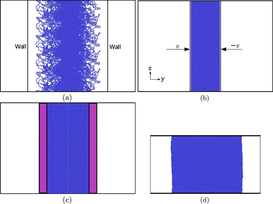
Figure 2. Steps in the process of preparing a sample with a well defined interface. (a) Repulsive walls are introduced after removing the pbc in the y-direction from bulk samples. (b) The repulsive walls are moved in to fold the protruding chains in and increase the density of the sample to that of the bulk. Two such samples are placed side by side in (c) and allowed to inter-diffuse. The sample is then quenched in (d) to a temperature below Tg and thereafter subjected to tensile deformation.
Download figure:
Standard image High-resolution imageAt this stage, with the repulsive walls in place, the sample is equilibrated at a pressure ph and temperature  in an NPT ensemble. The walls are removed after the equilibration at ph and Th is complete.
The equilibrated ensemble is now duplicated and the two copies are placed side by side (with a small gap of ∼2 Å) to create an interface perpendicular to the y axis. Further, a group of atoms at the two ends of the sample are fixed in order to create two 'rigid' regions that resemble, in an approximate sense, the infinite bulk that is attached to the two blocks created (see, figure 2(c), where the fixed monomers are coloured differently from the others). The welding process involves holding the interface at ph and Th for a holding time tw, during which entanglements are allowed to form across it. The evolution of entanglements across the interface is monitored.
After a holding time of tw, the sample is quenched at a rate  at ph to a temperature Tl < Tg. The rigid parts at the left and right ends of the sample are now pulled apart at a velocity v0, till the sample completely separates into two disjoint parts. In most cases, the failure occurs at the interface (see, figure 10). The difference in sizes between the samples in figures 2(c) and (d) is due to the fact that increase in density accompanies quenching.
Identifying and enumerating entanglements
We determine topological entanglements between segments of chains using the concept of the Gaussian linking number. The Gaussian linking number between two curves C1 and C2 was defined by Gauss (1877), and is defined as:

where  denotes a point on the curve Ci. For a pair of segments of polymer chains, the above integral can be determined by a robust algorithm involving solid angles defined by bond vectors (see, Ahmad et al 2020).
As discussed in detail in Ahmad et al (2020), topological entanglements between two chains I and J (shown in red and blue respectively in figure 3), can be enumerated by the method described below.
- 1.Firstly, we identify the atoms A and on chains I and J that lie closest to each other.
- 2.If the distance d between A and is less than dc, a predetermined threshold distance, the segments around these two points can potentially be entangled. Otherwise, the red and blue chains are not close enough to be entangled. In the present case, we have taken , which is about twice the largest value of the LJ parameter σ.
- 3.Next we calculate the linking number LkG between two segments BAC and C, where BA, AC and A are all segments with Nc atoms each. Thus, in most cases, linking number is determined for two neighbouring open segments containing 2Nc atoms each. The segments may be shorter if the end of either chain is encountered (as in the case of the segment on chain J).
- 4.If is more than Lc, the two segments are considered to be 'entangled'. The end points of the two segments and the value of the linking number are stored. Arbitrarily, atom A on chain I and on J are taken to be the location of the topological entanglement points on these two chains. The choice of the threshold Lc is somewhat arbitrary and based on our experience with the simple models. In this work we have taken Lc to be 0.4. Note that an entanglement can disentangle in the course of deformation.
- 5.We now leave these two segments out and search for the points (shown as D and in figure 3) which are the closest points outside the segment in the rest of the two chains. The same steps are repeated for two segments centred at D and , if the distance between them happens to be less than dc.


Figure 3. Definition of quantities involved in calculating LkG between segments of two chains I and J.
Download figure:
Standard image High-resolution imageThe above method enables us to identify all topological entanglements in the ensemble. Also, it is possible to follow individual entanglements during mechanical deformation of the samples and track disentanglement. It should be noted that the number of topological entanglements do not necessarily yield the rheological entanglement length as obtained from the plateau modulus of the melt. However, in this work, entanglements will be taken to mean only topological ones.
For the force field used and Lc = 0.4, earlier studies have reported topological entanglement length Ntopo of about 20. The rheological entanglement length Ne is about 80.
Results and discussions
The effect of the holding time tw on the strength of the thermally welded joint is demonstrated in figure 4. The time allowed for the interdiffusion to happen is varied from 0 to 60 ns at a holding temperature of Th = 500 K and pressure ph = 1 bar. In all the cases shown, the quench rate is  and the joint is pulled apart in the glassy state at a velocity
  . The response of the bulk sample deformed in tension at the same velocity is also shown for comparison. Recall that, we have not modelled scission of chains and so, pull out of chains is the only possible mode of failure. For a macromolecular ensemble with chains of 1000 monomers each, the strain at which pull out ensues is large (in reality chain scission would happen earlier) and so the bulk sample shows significant hardening even under tensile loading.
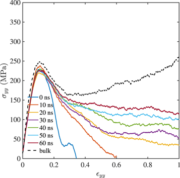
Figure 4. Effect of holding time tw on the strength of the thermally welded joint.
Download figure:
Standard image High-resolution imageIrrespective of tw, the maximum stress carrying capacity of the joint is the same, about 250 MPa, marginally lower than that of the bulk. This strength is determined by the non-bonded interactions between the two blocks placed in close proximity. However, careful consideration is needed before extrapolating this result to large surfaces in contact. Realistic, large surfaces are rough at the micrometre length scale and initial contact is established at a few asperities. Most parts of two realistic surfaces placed in contact are separated by distances that preclude them from interacting through non bonded interactions. This scenario is quite unlike the atomistically flat surfaces modelled here, which interact through non bonded forces all over the surfaces.
In some sense, the flat surfaces modelled here, mimic contact between parts of two asperities. Thus, our results show that two such asperities will locally bear stresses of the order of 250 MPa before they start to separate and this stress is independent of of tw. In other words, the force required to initiate separation of two large, rough surfaces depends on the number of asperities in contact or the roughness but not tw.
More interestingly, tw has a strong effect on the 'ductility' of the interface, where ductility is measured by the area under the σyy −  yy curves. Since chain scission is not modelled, this implies that interfaces held longer at Th are better at resisting chain pull out. This is shown in figure 5 where the variation of the entanglement density (normalised by the entanglement density of the bulk sample) in the y direction (i.e perpendicular to the interface located at y = 0) is plotted. The entanglement density close to the interface is very low at the onset i.e. tw = 0 ns. At tw = 10 ns, the trough in entanglement density around y = 0 has narrowed while entanglements from the interior of the bulk have moved towards the interface. At tw = 60 ns, the interface is hardly discernible because rearrangement of entanglements accompanying interdiffusion has almost equalised the entanglement density at the interface and the bulk. The most ductile interface results from the sample held at Th for tw = 60 ns, as is clear from figure 4. Similar equalisation of entanglement density with tw was observed by Ge et al (2013) (see, figure 2(a) of their paper) though they used a different technique for identifying entanglements.

Figure 5. Effect of holding time tw on the entanglement structure at the interface of the thermally welded joint.
Download figure:
Standard image High-resolution imageThe process of entanglement formation across an interface at high temperatures has been discussed by Wool et al (1989), based on the reptation model of a random coil chain. In their picture, chain ends (called minor chains in their paper) interdiffuse first to form entanglements across the interface. The number of new entanglements formed during the welding process between chains in one block with chains in the other can be tracked in our case. The quantity χi denoting the density of newly formed entanglements as a fraction of the entanglement density in the bulk sample is shown in figure 6(a) as a function of tw for Th = 500 and 800 K. The quantity χi increases linearly with tw at both temperatures.

Figure 6. The density of newly formed interfacial entanglements (as a fraction of the entanglement density of the bulk polymer) and the development of the interface thickness ai with tw are shown in (a) and (b) respectively. The location of the interfacial entanglement points are shown for tw = (c) 10 and (d) 60 ns. A histogram denoting the distance of the new interfacial entanglement points from the centre of the chain is shown in (e) for tw = 60 ns.
Download figure:
Standard image High-resolution imageThe interface width ai is the thickness upto which the newly formed entanglements penetrate into the bulk on either side. In figure 6(b), we calculate ai as the distance along y axis between the furthest new entanglements in y < 0 to the one in y > 0. The interface thickness can be measured experimentally by several techniques (e.g. Schnell et al 1998). Again, the interface width at both values of Th increases linearly with tw.
In our method of identifying entanglements (also see, e.g. primitive path analysis (Sukumaran et al 2005), Z1 (Kröger 2005), CReTA (Tzoumanekas and Theodorou 2006) and (Hoy et al 2009) for a comparison between these other methods), the actual location of the entanglement is somewhat arbitrary. We take it to be located at the point of closest approach between two entangled segments (like points A and  in figure 3). Given this definition, the black dots in figures 6(c) and (d) indicate the locations of the newly formed entanglements at tw = 10 and 60 ns respectively for the case with Th = 500 K. The spread of these dots in the y direction indicates the thickening of the interface with tw.
Also, as predicted by Wool et al (1989), most of the new entanglements are formed between two segments where at least one is an end segment. The histogram in figure 6(e), pertaining to tw = 60 ns and Th = 500, indicates the number of bonds from the chain centre at which a new entanglement is formed. It is clear from the histogram that most new entanglements involve the end 100−150 monomers of at least one of the two chains. Thus, large scale migration of complete chains from one side of the interface to the other is not needed for new entanglements to form. Most new entanglements are formed by the migration of chain ends.
Moreover, the entanglement distribution does not change much during the quenching process. Figure 7 shows the entanglement distributions at Th and the glassy temperature for two quenching rates. In the range of quenching rates that can be simulated, the entanglement distribution attained at Th 'freezes' to the glassy temperature, irrespective of the quenching rate.
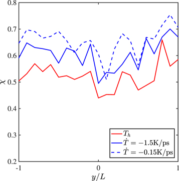
Figure 7. Effect of quenching rate  on the entanglement structure at the interface of the thermally welded joint.
Download figure:
Standard image High-resolution imageThe importance of the entanglement distribution attained at Th can also be demonstrated by studying the effects of Th and ph on the strength of the joint. In figures 8(a) the entanglement distributions for a waiting time of tw = 20 ns are shown. Closer the holding temperature is to Tg, deeper is the trough in χi at y = 0 indicating that fewer entanglements have formed across the interface. At 800 K, the distribution of χi has become almost uniform even for this short waiting time. The difference in the entanglement distributions reflect on the stress strain curves of the joint as shown in figure 8(b). The joints which were held at lower temperature are more brittle and have lesser strength than the ones held at higher. Even for a short waiting time of tw = 20 ns, the curve pertaining to Th = 800 K has almost completely regained the strength and ductility of the bulk sample. Thus, the time taken to attain near uniformity of the entanglement distribution at Th, when the entanglement distributions in the neighbourhood of the interface and bulk are almost similar, seems to be the single most important factor in determining the ultimate strength of the joint.
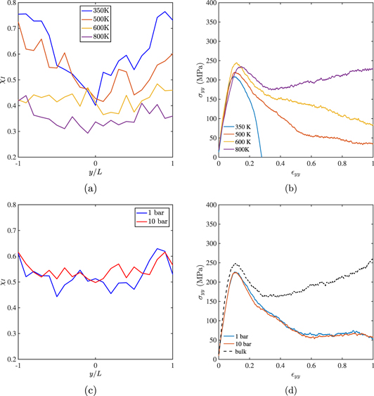
Figure 8. (a) The distribution of entanglements along y and (b) stress–strain curves in tension for interfaces held at various holding temperatures Th for a short holding time tw = 20 ns. For two holding pressures ph, the distribution of entanglements are shown in (c) for tw = 30 ns. The stress strain curves in tension for these two holding pressures are compared with that of the bulk in (d).
Download figure:
Standard image High-resolution imageOn the other hand, the effect of ph on the strength of the joint is marginal. The entanglement distributions for Th = 500 K and ph = 1 and 10 bar shown in figure 8(c) are almost identical for a waiting time of tw = 30 ns. The stress strain curves at the two pressures shown in figure 8(d) are also completely identical.
It is interesting to compare ai with some key length scales associated with the polymer chain. For homopolymer melts, the properties of the joint are indistinguishable from the bulk when chains have diffused by about their radius of gyration (Ge et al 2013). Assuming a freely jointed chain, polymer molecules in our ensembles (with 1000 monomers per chain) have radius of gyration Rg of around 20 Å. For all cases simulated, this is larger than the distance that centres of mass of the chains actually move. The quantity g2(t) denotes the averaged mean squared displacement of the centres of mass of the chains. In figure 9,  is plotted against
  at Th = 500 K. The average mean squared displacement of the chain centres of mass indicate that at 60 ns, chain centres have moved by a distance close to Rg, about 14 Å. This is manifested in the stress–strain response where, at 60 ns the sample has a stress strain response that is close to that of the bulk. In fact, for Th = 800 K, when the mean squared displacements are larger, samples held for tw = 60 ns do attain stress–strain responses almost same as that of the bulk. It seems therefore, that to attain joint strengths close to that of the bulk, chain displacements of the order of Rg must be allowed.

Figure 9. Average mean squared displacement of chain centres of mass g2(t) achieved after various waiting times tw.
Download figure:
Standard image High-resolution imageThe interface thickness in figure 6(b), also offers a measure of the depth of penetration of chains from one side of the interface to the other. For example, for the case with Th = 800 K and tw = 60 ns, the interface is about 15 Å wide on either side of the interface. This means that, for the topological and rheological entanglement lengths of 20 and 80 respectively, there are about 4–5 new topological and 1–2 new rheological entanglements formed on either side. This implies that, on an average, chain segments crossing the interface are tethered by at least one rheological entanglement on either side. This is consistent with the picture of an effective chain coupling across a polymer-polymer interface proposed by Silvestri et al (2003).
The nature of adhesive failure at the interface also depends on the entanglement distribution. For distributions with deep troughs at the interface (obtained for very short tw or low Th), the failure is brittle as shown in figure 10(a). Craze-like fibrillation occurs at the interface when tw is increased and the joint becomes more ductile (figure 10(b)). At high enough Th and long tw, the joint becomes as strong as the bulk. As shown in figure 10(c), in this case, failure is no longer concentrated at the interface and occurs by cavitation and fibrillation all over the sample.

Figure 10. Nature of adhesive failure is shown for (a) very short tw and low Th, (b) intermediate tw and (c) long tw and high Th.
Download figure:
Standard image High-resolution imageThe energy per unit interface area Gc is a measure of the effect of the entanglements formed across the interface. The toughness Gc of the interface can be measured through standard fracture experiments on lap shear or double cantilever beam (DCB) samples. In our MD simulations, the interface is pulled apart in tension at extremely high loading rates. The energy required to cause failure, per unit interface area, under tension at these rates, is not identical to the Gc values obtained from standard fracture tests. As noted by Léger and Creton (2008) if the two blocks in contact interact through van der Waals interactions only, the estimated Gc turns out to be 2–3 orders of magnitude lower than what is measured from experiments. Experimental values of Gc of thermally welded symmetric polymers are in the range of 10−100 J m−2 (Schnell et al 1999) from DCB tests. Theoretical estimates of the adhesion energy increase when there are a large number of 'connector chains' entangling with the polymer networks on either side of the interface.
In this work, the quantity Gc, obtained by dividing the total energy required to completely separate the two polymer blocks by the area of the interface, should be interpreted in light of the discussion above. The fracture toughness obtained from say, tests on DCB specimens, involves large contributions from crack tip plasticity and other dissipating mechanisms operating over significantly larger length scales4 than the ones at which the MD simulations are conducted. Thus, the Gc reported from these simulations are invariably smaller than experimental ones. Also, failure in our simulations is only due to chain pull out as scission is not allowed.
Figure 11(a) shows the effect of holding temperature Th (for tw = 10 ns) on Gc. For a low Th = 350 K, at tw = 10 ns, almost no entanglements form across the interface (see, figure 8(a)), and the interface is extremely brittle (as is also evident from the clean fracture observed in figure 10(a)). Only non-bonded interactions contribute to the extremely low Gc. From our simulations, it seems that Gc increases linearly with the holding time Th.

Figure 11. Plots showing the variation of Gc with (a) Th at tw = 10 ns, (b) interface thickness ai obtained at Th = 500 K, (c) tw at Th = 500 K, and (d) no. of monomers per chain N.
Download figure:
Standard image High-resolution imageWe have already shown that the interface width ai is a monotonically increasing function of Th. This fact can be used to connect our simulation results with experimental measurements of Gc. Experimentally (e.g. Schnell et al 1999, Brown 2001), the value of Gc for polystyrene-polystyrene interfaces show a regime of slow rise followed by one of rapid growth and finally, slow saturation to the bulk toughness when plotted against the interface with ai. Values of Gc from our simulations, when plotted against ai in figure 11(b), shows a slow rise followed by steeper increase. However, our simulations are not long enough to capture the region of slow saturation seen in experiments.
A further comparison of the trends in Gc with experiments is possible when it is plotted against the waiting time tw. In figure 11(c), Gc is plotted against tw at Th = 500 K. Results from lap shear tests show that  (e.g. Akabori et al 2006) before it becomes independent of tw at very large values of tw. Similar results on polystyrene-polystyrene interfaces are reported by Schnell et al (1999), where Gc obtained from DCB tests are plotted against reduced time at reference temperature of 393 K. In comparison to these experimental results, the range of tw in our simulations is small. While the saturation observed by Akabori et al (2006) at large tw, is beyond the capability of the MD simulations,
  does seem to provide a reasonable fit to the data even at the short time scales accessible to the MD simulations.
Finally, the effect of chain length N on Gc is shown in figure 11(d). We have conducted simulations for four values of N with tw = 10 ns. For chains that are shorter than the rheological entanglement length Ne and close to Ntopo, the strength is only governed by the van der Waals interaction. Hence, for N = 20, the value of Gc is very low (even less than the N = 1000 sample held at Th = 350 K for tw = 10 ns in figure 11(a)). A jump in toughness occurs when N > Ne and thereafter Gc increases almost linearly with N. Variations of interface toughness with molecular weight for symmetric interfaces, to the best of our knowledge, has not been explored experimentally. But, from results on asymmetric interfaces (e.g. Cole et al 2003), a plateauing of the toughness is expected at high N. The plateau appears due to a switch from a failure dominated by chain pull out to one dominated by chain scission. It does not appear in our simulations as chain scission has not been modelled.
Conclusions
With a view to understand the effect of process parameters on the mechanical strength of thermally welded joints between two similar monodisperse polymers, we have conducted a series of MD simulations on a generic macromolecular ensemble. The strength of the joint depends very strongly on the number of chains that diffuse from one side of the interface to another to get entangled there. Most of such entanglements are formed with chain ends that are the earliest to diffuse across. Strengths approaching that of the bulk can be attained even when chains have diffused by amounts that are smaller than their radii of gyration. The following conclusions can be drawn from the results reported:
- 1.The most important process conditions affecting the strength and ductility of a symmetric interface are the holding temperature Th and the time tw. Both of these can lead to an increase in the number of entanglements formed across the interface which in turn, leads to increase in the interface width.
- 2.The effects of applied pressure and quenching rate have marginal effects on the strength and ductility of symmetric interfaces.
- 3.The interface width scales as ai ∼ tw and the interface toughness. Also, the simulations suggest that Gc ∼ N, for .
- 4.As the response of the joint tends towards that of the bulk, its mode of failure under tension goes from clean brittle fracture, to fibrillation at the interface followed by delocalised cohesive failure with cavitation occurring all over the bulk.


Footnotes
- 4
Plastic zone sizes are of the order of Gc/σ0 where σ0 is the maximum stress the joint can bear.