
Abstract
Following the work of Schwinger (1961 J. Math. Phys 2 407), we present a general method for deriving quantum response functions on a closed-loop contour in the complex time plane. We focus on optical response functions of linear to third order and demonstrate by projecting contour time onto the real axis how they connect to Liouville space pathways. This work highlights the close connection between the Keldysh contour and the double-sided Feynman diagrams used in nonlinear optical spectroscopy. In addition, we give a Keldysh contour derivation of the Marcus equation for electron transfer.
Export citation and abstract BibTeX RIS
1. Introduction
Following the work of Schwinger [1], we develop quantum response theory on the Keldysh contour [2–6]. Focus is on the nonlinear response functions and their application within coherent multidimensional spectroscopy. The discovery of long-lived oscillations in coherent multidimensional spectroscopy of photosynthetic antenna systems [7–9] and the ensuing mechanistic debate demonstrate the need for detailed theoretical work [10]. In particular, understanding the non-Markovian dynamics of an assembly of chromophores embedded in a structured environment is of paramount importance. The use of non-equilibrium Green's functions (NEGFs) immediately avails us of the general and flexible techniques of quantum many-body physics, which promises to handle a well-balanced compromise between high-quality quantum dynamics and atomistic description of the molecular structure. Furthermore, it offers the perspective of a unified theoretical description of current and light in combined experiments such as scanning tunnelling microscopy/tip-enhanced Raman spectroscopy experiments.
NEGFs [2–6, 11], which have experienced a revival over the past two decades, are largely used in quantum transport theory [6, 11–13], describing current in mesoscopic nanostructures, quantum dots, carbon nanotubes and single molecules. Inspired by the intimate connection between electron transfer and electron transmission [14, 15], Yeganeh et al derived the Marcus equation of electron transfer from the Landauer equation of molecular electronics, thus foreshadowing a direct NEGF-based derivation of the Marcus equation [16].
The use of NEGFs in nonlinear spectroscopy appears only sporadically in the literature [17, 4] (and references in [4]). Early work includes application to x-ray photo-emission [4, 18], Auger emission [19] and x-ray Raman spectroscopy [20]. Mukamel, who with his landmark monograph entrenched the use of Liouville space pathways in the analysis of multi-dimensional spectroscopy [21], has pointed out the close link between double-sided Feynman diagrams (that illustrates density matrix propagation) and the Keldysh contour. He has developed a partially time-ordered wavefunction formulation on the Keldysh contour, which is used, in conjunction with the Liouville space formulation, to analyse optical and x-ray spectroscopy experiments [22–27].
We develop the general theory first in section 2. The optical response functions of linear, second and third orders are examined in great detail. We project contour time on the Keldysh contour onto the real time axis to connect to Liouville space pathways. This augments the partially ordered wavefunction formulation, which now constitutes an independent alternative to the Liouville space formalism. The work exposes a clear connection between the Keldysh contour and double-sided Feynman diagrams. In addition, we demonstrate a Keldysh-contour-based derivation of the Marcus equation of electron transfer.
2. Response theory
In this section, we will develop response theory on the Keldysh contour. The connection to Kubo's well-known approach will be made in section 3. We consider a quantum system, such as a single molecule or an aggregate of chromophores, described by a Hamiltonian, H0, and seek to monitor the expectation value of a system operator,  , while the system is exposed to a time-dependent perturbation,
  , introduced at time t0. A total Hamiltonian reads

with ϑ(t − t0) being the Heaviside step function. In the absence of the perturbation, we can write


where  is the density matrix. The forward and subsequently backward propagation on the real axis can be recast as forward propagation on a Keldysh contour—a closed-loop contour that begins at t0 extends to t and returns to t0. Perturbations are introduced via a contour-ordered exponential
where Tc[...] is the contour ordering operator. The operator  operates at time t and is thus included in the contour ordering. The expectation value now reads

The power series expansion of the contour-ordered exponential suggests writing the corrections to the unperturbed expectation value (n = 0) as an infinite series:
Making the identification with equation (7), an explicit definition of the nth-order correction is obtained:
In the following, we shall examine the correction of the first through third order in some detail.
3. Optical response functions
The optical polarization,  , is key when discussing optical properties of materials. When the chromophore is much smaller than the wavelength of the light, which is indeed the case for optical spectroscopy in the visible spectrum for organic chromophores, we can work in the dipole approximation, where the polarization operator is approximated by the dipole moment operator,
  . We write the molecule–light interaction as

where E(t) describes a time-dependent electric field. Notation describing the vector properties of the dipole moment and field, as well as field polarization, has been suppressed.
3.1. Linear response function
The correction to the dipole moment to linear order in the perturbation is given by
The contour time ordering of the two dipole operators,  and
and  , is written out explicitly using Heaviside step functions
and the linear response term now splits into two:
The two loop diagrams contributing to linear response (representing equations (13) and (14)) are depicted in figure 2. (Strictly speaking, we identify each diagram with a Liouville space pathway; see below.) Physical time runs on the real axis, where we focus on the interval between times t0 and t. The contour introduced via the contour-ordered exponential comprises a closed loop in the complex time plane (see figure 1). We take contour 'time' to begin at t0 and to propagate clockwise around the contour. The contour crosses the real axis at the observation time t and propagates back to t0. The first term, equation (13), has τ1 before t on the contour; thus, the scattering event occurs on the upper branch of the loop contour and is represented by the diagram to the left in figure 2. Conversely, term two has the scattering occurring at a point τ1 occurring after t, and τ1 is thus marked on the lower branch in the right diagram in figure 2. To project contour time onto physical time, we follow, in spirit, the strategy laid out by Langreth [4]. Under the general assumption that the integrand has no poles within the loop diagram, we invoke Cauchy's integral theorem to continuously deform the contour. Having pinned the contour to the real axis at times t0 and t, we tighten the loop contour. On the upper branch of the contour, contour time morphs continuously into physical time and we obtain the limits ∫cdτ → ∫tt0dτ on the time integrals. For the lower time contour, we obtain ∫cdτ → ∫t0tdτ. Flipping the limits of the time integration on the lower branch at the cost of a sign ( ), we could obtain Kubo's expression from equations (13) and (14):
We note that by working with the loop contour we avoid the need for commutators. Disregarding correlations in the initial state we let t0 → −∞, also we extend the integration to infinity by introducing a Heaviside step function. Substituting the time variable t1 = t − τ1,
Define the linear response function, S(1)(t1), indirectly, via the convolution integral
which gives us the expression
The dependence on t is only apparent, since when disregarding correlations in the initial state, we secured time translation invariance, and we can choose t − t1 = 0 to obtain
The Heaviside function explicitly ensures causality. The two terms are complex conjugated. Defining  we can write
Complex conjugation corresponds to the reversal of contour time; for the loop diagrams this amounts to reflection in the real axis.

Figure 1. A Keldysh contour from t0 to t, with a scattering on the upper branch at time τ1. We have inflated the Keldysh contour into a loop diagram for clarity.
Download figure:
Standard image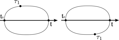
Figure 2. Loop diagrams representing the two Liouville space pathways of the linear response function.
Download figure:
Standard image3.2. Second-order response function
The second-order correction to the dipole moment is given by
Expansion of the contour ordering of n + 1 operators gives (n + 1)! terms (in this case 3! = 6):


We group these terms according to the position of  . Consider first the n! (in this case 2! = 2) terms where t occurs first on the contour (we will refer to these terms as III):
When we tighten the loop contour the contour 'times' τ1 and τ2 lie on the lower, anti-time-ordered branch of the Keldysh contour.
For each of the k (here 2) contour 'times' on the lower branch, we flip time, i.e. the limits of the 'time' integration, at the cost of a sign. We obtain an overall factor of ( − 1)k (here 1). The n! terms now differ only by the permutation of the integration variables. We choose one ordering and eliminate the factor of  . To connect to experiments, we identify the specific ordering of the dummy time variables with ordering in physical time:
We let the reference time t0 go to the infinite past  and introduce a second step function ϑ(t − τ2):
Now we make the substitution ti = τi + 1 − τi (τn + 1 ≡ t) of the time variables τi. The new variables ti refer to the time intervals between scattering events. We note that  ; hence, the Jacobian of the variable substitution equals unity, |Jn| = |( − 1)n| = 1:
Define the second-order response function indirectly by
So far, we have obtained the contribution from the term III:

where  . Next consider the n! terms with one time before t (we refer to them as II)
We arrive at a single term with no relative order of the scattering times τ1 and τ2. We split this term in two by introducing two Heaviside functions: 1 = ϑ(τ2 − τ1) + ϑ(τ1 − τ2). Subsequently, we swap the two dummy time variables in the second term to obtain two terms (IIA and IIB):

Making time substitutions as above and writing only the contributions to the response function, we have


Defining two of the Liouville space pathways as


the response function can be written as
Each of the contributions is given by


The four Liouville space pathways are shown in figure 3. We started out with (n + 1)! terms, which were grouped into (n + 1) groups of terms that turned out to be identical, eliminating the factor of n! from the contour-ordered exponential. To have a specific time ordering, we split each term having k times on the lower branch into  individual terms, for a grand total of
  terms, a result we could have anticipated since we distribute n times on two branches of the contour.

Figure 3. Loop diagrams for quadratic response.
Download figure:
Standard image3.3. Third-order response function
Many coherent spectroscopy experiments performed today relate to the third-order response function, S(3)(t3, t2, t1), and we shall briefly go through its derivation. Specifically, we shall focus on how to stack the decks when shuffling two time orderings, one on each branch of the Keldysh contour, into a single time ordering in physical time. We shall demonstrate, by explicit derivation, which Liouville space pathway is contributed by each loop diagram:
A full expansion of the contour ordering gives (3 + 1)! = 24 terms, of which we write four representative terms (that we will refer to as terms I–IV):
Consider term III, where one time occurs before t, and thus lies on the upper branch of the loop diagram. The remaining two times lie on the lower contour. Deforming to the Keldysh contour, we obtain


Note the sign change in the argument of the remaining Heaviside function. This is a consequence of contour ordering being deformed to anti-time ordering, and the subsequent time flip. We now have three times on the real time axis, but only two of these are ordered. To relate to physical time, full time ordering is desired. We split the term into three terms, where the time from the upper branch occurs before, in between, or after the two ordered times from the lower branch (we shall refer to these as IIIA, IIIB and IIIC):
As discussed above, a term with k times on the lower branch can be split into  terms with specific time ordering. Define the third-order response function indirectly by
Each term, for example IIIA, is accompanied by five identical terms, thus eliminating the factor  . We substitute times to obtain
Defining four Liouville space pathways as
the response function is given by
The contribution from the various terms are as follows:


The four remaining terms are related to the first by complex conjugation:


The eight Liouville space pathways contributing to the third-order response function are depicted in figure 4. With the strategy laid out in these sections, one could now derive expressions for the 2n Liouville space pathways contributing to the nth-order response function, and subsequently evaluate the corresponding correction to the dipole moment operator:
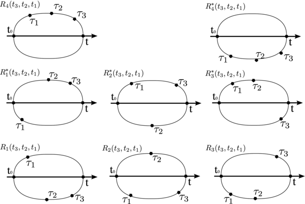
Figure 4. Loop diagrams for third-order response.
Download figure:
Standard imageAs the avid reader has noted, the loop diagrams relate to the double-sided Feynman diagrams encountered in nonlinear optical spectroscopy. Imagine the loop diagram in figure 5 to be rotated at 90°. Note that the information about the phases of the electrical field implied by the corresponding arrows are not given in the loop diagram.
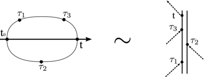
Figure 5. Loop diagrams relate to double-sided Feynman diagrams.
Download figure:
Standard image4. The Marcus equation
The Marcus equation describes non-adiabatic electron transfer and is widely used to describe electron transfer in chemistry and biology. The theory was developed in the late 1950s by Marcus [28, 15]. A notable prediction of the theory, subsequently confirmed by experiment, was the existence of a Marcus inverted regime of decreasing electron transfer rate.
Recently, Yeganeh et al derived the Marcus rate starting from the Landauer equation for electron transmission. They predicted the possibility of a direct NEGF-based derivation. With the response theory developed in section 2, we are ready to do just that.
4.1. Fermi's golden rule
As a prelude, we shall consider transitions in a purely electronic system and obtain Fermi's golden rule as a linear response function. Consider a two-level system, H0 = εa|a〉〈a| + εb|b〉〈b|, initially prepared in the state |a〉,  . At time t0, a coupling between the states, V = Vab|a〉〈b| + Vba|b〉〈a|, is introduced and we monitor the rate of transition
  , calculated using the Liouville equation:
Now, evaluate the transition rate to first order in the coupling (using expression (17)):
We recognize Fermi's golden rule and note that the rate is independent of time t, since the perturbation is not associated with an external field.
4.2. The Marcus equation
Mathematically, the derivation of the Marcus equation is a slight generalization of the derivation of Fermi's golden rule. Considering the two-level system coupled to a single bosonic mode,
Shift the bosonic mode ( and
and  ) to obtain

where we have defined  , Δv = vb − va and
  . We use the transition operator of equation (82) and choose
  with
with  . The transition rate to linear order in the coupling is given by
With the merging of the two terms, we are back on the beaten track and the final steps are found in multiple textbooks [15, 6]. The integrand factorizes as

The correlation function Cba(t1) evaluates to

where n(ω) = (eβℏω − 1)−1 is the Bose distribution function. In the limit where the correlation function is short-lived,  , the exponential functions in the exponent can be expanded to second order in ωt1 and the integral becomes a Gaussian integral. We obtain the celebrated Marcus equation
where  . The Keldysh contour derivation given here turned out to be no more than a response function derivation. The methodology used, however, applies also to higher order corrections.
5. Conclusion
The evaluation of expectation values on a loop contour in the complex time plane was introduced by Schwinger in 1961. We have presented a method for explicitly calculating nonlinear response functions on a loop contour.
For the specific case of optical response functions, we undertook a detailed derivation. Contour time was projected onto the real time axis, which led to the connection to the Liouville space pathways. The derivation demonstrates the close connection between the Keldysh contour and double-sided Feynman diagrams, and paves the way for the use of many-body techniques in nonlinear optical spectroscopy.
As another application of response theory, we provided a Keldysh contour derivation of the Marcus equation of electron transfer.
Acknowledgments
We gratefully acknowledge financial support of the Swedish Science Council, the Knut and Alice Wallenberg Foundation, Swedish Energy Agency and Crafoord foundation. TH gratefully acknowledges a travel grant from the Danish Chemical Society.