

Abstract
Two-layer systems heated from above with buoyancy as the driving force may show a rather paradoxical instability mechanism called anticonvection. This transition from a conductive to a convective state is determined by the interface as well as bulk properties (buoyancy forces) of the two fluids. In this paper, we derive the equations for perturbated fields from the basic hydrodynamic equations. An analytical expression for the control parameter at threshold is presented for a vertically infinitely extended system. Further on, we perform a linear stability analysis of a vertically bounded mercury–water system and compare these results with the vertically infinitely extended system. Finally, we show some three-dimensional simulations of the fully nonlinear equations and the resulting patterns for an anticonvective mercury–water system.
Export citation and abstract BibTeX RIS
Communicated by E Knobloch
1. Introduction
The famous convection experiments performed by Bénard (1900, 1901) in 1900 initialized a great deal of effort to understand and describe convective instabilities in vertically heated fluid systems over the last century. Even though this convective instability is induced by thermocapillarity at the free surface, buoyancy as a driving force may also be seen in the framework of Bénard's experiments. The occurrence of the Bénard roles was explained theoretically with thermocapillary forces (Bénard–Marangoni) as well as with buoyancy forces (Rayleigh–Bénard) in early works. However, these investigations considered the upper gas layer as passive, and analyses were performed mainly in one-layer models. It is natural to extend the investigation of these systems to configurations with more than one layer.
Here we focus on systems heated from above. Experiments for different fluid combinations were performed by Juel et al (2000) and showed the rich variety of pattern formation in two-layer systems. Note that experimentally both thermocapillary and buoyancy effects are present. Theoretical investigations of the pure Bénard–Marangoni instabilities in two-layer systems in the frame of amplitude equations were performed by Colinet et al (1996) and showed also a rich variety of bifurcations. Note that these calculations were done with the Marangoni effect only and were done close to a codimension two point.
Multi-layer systems heated from above with buoyancy effects alone were not investigated until 1964. It was argued that multi-layer systems driven by buoyancy effects become only unstable on applying heating from below. Potential energy release was seen as being impossible for heating from above and consequently the system rests in its conductive state. However, Welander (1964) showed in 1964 that a two-layer system heated from above can overcome this stabilizing mechanism. He used the expression anticonvection for that paradoxical kind of instability. Linear investigations of vertical bounded (finite) systems were done by Gershuni and Zhukhovitskii (1980) in 1980. They found the range of material parameters in which anticonvection can occur. First results of nonlinear investigations were also done at this time by Simanovskii (1980) and Gershuni et al (1981). Since anticonvection arises due to various interactions at the interface, only special fluids allow for an instability. However, Ingel (1997) revealed that an (infinitely extended) water–air system is anticonvectively unstable if phase transitions (evaporation) or the salinity of water is taken into account. Nepomnyashchy et al (2000) and Nepomnyashchy and Simanovskii (2001) showed that every (bounded) two-layer system can become anticonvectively unstable for heat sources or sinks at the interface (e.g. evaporation, chemical reactions and so on). Furthermore, they proposed an experimental realization of interfacial heating (infrared light sources for a silicon oil–ethylenglycol system; (Nepomnyashchy and Simanovskii 2001)). Investigations on combined actions of buoyancy and thermocapillarity with heat sinks and sources at the interface performed by Nepomnyashchy and Simanovskii (2002) in 2002 showed that a distinction between thermocapillary and anticonvective domains is possible. Also Simanovskii et al (2009) dealt with the joint action of both effects and revealed some new types of nonlinear traveling waves. The effects of an imposed horizontal temperature gradient in anticonvective systems were reported by Simanovskii et al (2002) and may be considered to give an insight into more realistic scenarios. Note that experiments for two-layer Rayleigh–Bénard systems heated from above in the context of anticonvection have not be done so far, since surface tension effects can cover the anticonvective instabilities (see, e.g., Degen et al (1998) and references therein). However, all the above-mentioned theoretical and numerical investigations indicate possible setups and parameter regimes for future experiments.
The increased computer power available nowadays allows direct numerical three-dimensional (3D) investigations for two-layer systems. For instance, Boeck et al (2002) showed pattern formation in two-layer systems driven by surface tension effects. Therefore the numerical investigation of pattern formation in anticonvective systems is in the offing. Full 3D simulations of anticonvective systems can be found in Merkt (2005) and Boeck et al (2008).
In this paper, we perform analytical as well as numerical investigations of a two-layer system with buoyancy effects heated from above. First, we derive the governing equations for the perturbated field quantities from the basic hydrodynamic equations. Then we perform numerically a linear stability analysis of a vertically bounded system. This allows us to reveal the effect of the boundaries on the system. Our linear results are compared with the analytical expression for the marginal control parameter of a vertically infinitely extended system. The derivation of this analytical expression can be found in the appendix. Further on, we show 3D results of direct numerical simulations of an anticonvective system bounded by rigid plates at the top and bottom. We focus on a mercury–water system for several reasons. On the one hand, the large number of free parameters complicates general predictions for two-layer systems, even numerically. Furthermore, mercury–water setups are the only known systems which show anticonvection without heat sources at the interface. On the other hand, experiments can be performed more or less easily for a mercury–water system.
The mechanism of anticonvection has to be considered as a subtle combination of effects in the bulk and at the interface. Consider a system with large thermal expansion coefficient (α1 > α2) and large thermal diffusivity (κ1 > κ2) in the lower layer (figure 1). Due to buoyancy a positive temperature fluctuation close to the interface in the lower layer forces the fluid to move to the interface (point 1). At the interface, viscous coupling induces a (passive) convective motion in the upper layer (point 2). Since buoyancy and thermal diffusivity in the upper layer are small, hot fluid from above is transported to the interface (i.e. the upper layer serves as a heat supplier and is called a type I system; (Nepomnyashchy et al 2000)). Thermal coupling allows then for heat transfer to the lower layer (point 3) and, finally, thermal diffusion (point 4) can amplify the primary positive temperature fluctuation in the lower layer. Note that this is an essentially different instability mechanism than the usual Rayleigh–Bénard instability driven by buoyancy alone.
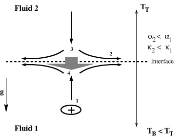
Figure 1. Sketch of an anticonvective system. The thermal expansion coefficient α1 and the thermal diffusivity κ1 of the lower fluid are larger than those of the upper one. A positive temperature perturbation in the lower layer close to the interface leads to a convective motion due to buoyancy (1). Viscous coupling induces a passive convective flow in the upper layer (2). Therefore hot fluid is transported to the interface (3). Thermal coupling and large thermal diffusivity can amplify the primary perturbation (4).
Download figure:
Standard imageTo summarize, anticonvection can arise if at least four timescales match: buoyant timescale in the bulk, viscous timescale, thermal timescale and heat flux timescale at the interface.
2. Governing equations
Two-layer systems with layer thickness d1 for the lower fluid and d2 for the upper fluid (ratio d = d2/d1) are described by the Navier–Stokes equations, energy equation and incompressibility condition for each fluid layer:


The subscripts i = 1,2 denote the lower and the upper fluid, respectively. ρi are the densities, νi the kinematic viscosities, g the acceleration due to gravity, κi the thermal diffusivities and ez the unit vector in the z-direction. vi are the velocity vectors, Pi the pressures and Ti the temperatures.
Rigid boundaries at the bottom and top of the system provide (z = 0 and z = d1 + d2)


with Tb and Tt being the temperature of the lower and upper plates, respectively. The conditions ∂zviz = 0 result from both vi = 0 and the continuity equations (1c). We consider an undeformable interface. Therefore the interface conditions can be written as (z = d1)


with λi for thermal conductivities.
In the following, we use the Boussinesq approximation, i.e. all material parameters are independent of temperature except for densities in the gravity term (equation (1a)). A linear expansion provides


where Ti is a (stationary) reference temperature of the interface. ρ10 and ρ20 are reference densities in fluid 1 (at Tb) and fluid 2 (at Ti), respectively. α1 = −1/ρ10·∂ρ1/∂T|Tb and α2 = −1/ρ20·∂ρ2/∂T|Ti denote the thermal expansion coefficients in fluids 1 and 2, respectively.
We use the nondimensional variables

where ΔT = Tb − Tt denotes the temperature difference of the bottom and top plates. We find that, for the stationary nondimensional temperature profile (we dropped the tildes),


where


are nondimensional temperature gradients in fluids 1 and 2, respectively. The conductive state is described by

Finally, we obtain from equations (1a)–(1c) for the perturbated quantities (u for the velocity, θ for the temperature and p for the pressure) a set of equations


Due to the Boussinesq approximation in each layer, the thermal expansion coefficients αi appear in the bulk equations (hidden in R).
The boundary conditions (2a) and (2b) transform to


and from equations (3a)–(3c) the interface conditions at z = 1 read


The necessary material parameters of the system are the ratios of the layer thicknesses d = d2/d1, the densities ρ = ρ2/ρ1, thermal conductivities λ = λ2/λ1, thermal diffusivities κ = κ2/κ1, kinematic viscosities ν = ν2/ν1 and the thermal expansion coefficients α = α2/α1.
Further on, two dimensionless numbers result:


where the Rayleigh number R is the control parameter of the system.
2.1. Linearized equations
Equations (9a)–(9f) and the corresponding boundary and interface conditions (equations (10a) and (10b) and (11a)–(11c)) allow formulation as a general linearized eigenvalue problem. Therefore a normal mode ansatz for both fluids is used in the usual manner


where  ,
,  ,
,  and χ is the growth rate. The velocities uxi and uyi are eliminated using the incompressibility conditions equations (9c) and (9f)). The phase shift −iπ/2 in equation (13b) ensures real equations in the following. Subsequently applying the curl and neglecting nonlinearities provides linear equations for fluid 1 (see also Chandrasekhar (1961) and Merkt and Bestehorn (2003))


and for fluid 2


The boundary conditions (10a) and (10b) turn out to be

and the interface conditions (11a)–(11c) read


3. Numerical integration of the bounded system
3.1. Linear results
The general eigenvalue problem of the bounded system (equations (14)–(16)) for the growth rate χ is solved numerically.
First, we investigate the influence of the ratio of thermal expansion coefficients on the instability. Figure 2 shows the marginal stability line in the R–α-plane for d = 1 with parameters from table 1. Decreasing α leads to a smaller absolute value of the critical Rayleigh number Rc. Due to the anomaly of water the thermal expansion coefficient of water α2 will be negative for temperatures below 4 °C. Therefore we suppose a monotonically decreasing function for α2 and also for the ratio α = α2/α1 with decreasing temperature. In the following, we use α = 0.1144. This is reasonable since experiments can be performed with an upper plate temperature less than 20 °C.
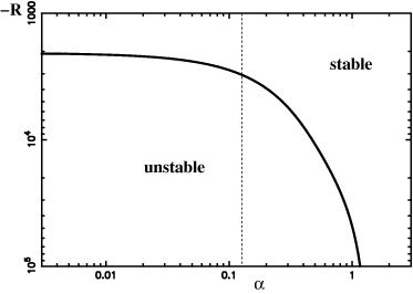
Figure 2. Contour plot of the marginal state in R–α representation. Decreasing the ratio of thermal expansion coefficients α decreases the absolute value of the critical Rayleigh number Rc. The dashed line indicates the ratio used for further investigations.
Download figure:
Standard imageTable 1. Material parameters of a mercury–water system at 20 °C. Due to the anomaly of water, the ratio α decreases for decreasing temperatures. We take α = 0.1144 for our investigations and assume the other parameters to be constants.
| Mercury (lower layer) | Water (upper layer) | Ratio | |
|---|---|---|---|
| Density ρ (gm−3) | 13.546×10⁶ | 0.9982×10⁶ | 0.0737 |
| Viscosity ν (m2 s−1) | 1.15×10⁻⁷ | 1.0×10⁻⁶ | 8.696 |
| Thermal diffusivity κ (m2 s−1) | 4.35×10⁻⁶ | 1.43×10⁻⁷ | 0.0328 |
| Thermal expansion α (K−1) | 1.81×10⁻⁴ | 2.07×10⁻⁴ | 1.144 |
| Thermal conductivity λ (W (mK)−1) | 8.2 | 0.598 | 0.073 |
| Prandtl number Pr | 0.026 | 7.0 |
Figure 3 (solid thick line) shows the marginal Rayleigh number R versus k for different layer ratios d. We find that the critical Rayleigh number Rc ≈ −2950 and the critical wave number kc ≈ 1.33 for d = 1 (thick black line). Surprisingly, this critical wave number kc can be stabilized by stronger heating (increasing the control parameter −R). This is in contrast to the normal Rayleigh–Bénard instability (heating from below) where the marginal R–k diagram shows a parabolic shape (i.e. an unstable wave number stays unstable by increasing the control parameter). Further on, we show the analytical expression

(see equation (A.11) in the
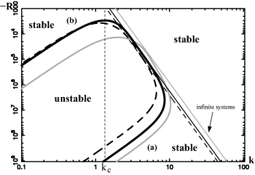
Figure 3. Contour plot of the marginal state Rc versus the wave number k. The thick black line is the marginal state with d = d2/d1 = 1 (dashed: d = 1.5; gray: d = 0.43). Every unstable wave number is stabilized for a large enough increase of |R| (i.e. increasing the applied temperature gradient). The thin lines are the marginal states for an infinitely extended system in the z-direction where we used the expanded expression for Rc∝ − k4 (see text). The boundaries are getting important for both small and large wave numbers.
Download figure:
Standard imageSmall wavelengths (a) cause two convection roles on top of each other in the upper layer. Therefore the heat transport from the upper boundary to the interface is decreased. Large wavelengths (b) inhibit a passive convective motion in the upper layer since the horizontal motion along the interface is slowed down and finally stopped by viscosity. Note that the latter mechanism already occurs in the 'normal' Rayleigh–Bénard convection.
Figure 4 shows the eigenfunctions in the unstable domain for different wave numbers k using the same Rayleigh number (R ≈ −2980). For the critical wave number (solid line) the eigenfunctions of the velocity and the temperature perturbation are positively correlated in the upper layer (sign(uz) = sign(θ)), i.e. potential energy is released in the upper layer. The eigenfunctions are changed essentially with increasing or decreasing the wave number, respectively. Firstly, the stabilization for small wavelengths (k > kc, dashed line) for finite extensions in the z-direction is caused by the appearance of an anticorrelated region of uz and θ at the boundary of the upper fluid, namely sign(uz) = −sign(θ). This reduces the release of potential energy in the upper layer. A further increase of k spreads this anticorrelated region and destabilization is not possible for a large enough k. Note that an increase of the absolute value of the control parameter has the same effect for any fixed wave number k. Consequently, a large enough −R stabilizes every wave number k and explains branch (a) in figure 3.
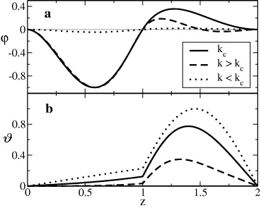
Figure 4. Eigenfunctions (φ, ϑ) of (a) the velocity uz and (b) the temperature θ with R = 1.01Rc ( = 0.01) for k = kc (solid line), k > kc (dashed line) and k < kc (dotted line). The growth rate χ > 0 for all eigenfunctions (i.e. unstable regime).
Download figure:
Standard imageSecondly, for large wavelengths (k < kc, dotted line, see also branch (b) in figure 3) the eigenfunction of the velocity uz tends to zero. Therefore the control parameter of the system has to be increased for large wavelengths.
3.2. Nonlinear results
In this subsection, we solve the fully nonlinear equations (9a)–(9f) numerically. We use periodic boundary conditions laterally and a semi-implicit pseudospectral method. The discretization in the z-direction is done with finite differences. The stationary state is perturbed by small randomly distributed fluctuations.
We redefine the control parameter as

and we use a 128 × 128 × 20 grid for each layer.
Figure 5 shows patterns of stationary states at t = 3000 and t = 1000 for = 0.15 and = 0.4, respectively. We use parameters of a mercury–water system (see table 1) with d = 1, α = 0.1144 and an aspect ratio of Γ = 18.8 (i.e. four times the critical wavelength). A transition from hexagons to squares takes place by increasing the control parameter . We have to note that squares are not found in the simulations of Boeck et al (2008). However, these transitions from hexagons to squares (and even weak turbulent regimes) are well known for single-layer Bénard–Marangoni convection via increasing the control parameter (Merkt and Bestehorn 2003).
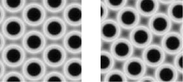
Figure 5. Contour plot of the interface temperature perturbations (stationary stable state). Dark areas indicate negative and light areas positive temperature perturbations, respectively. We use parameters from table 1 with d = 1, α = 0.1144, 128 × 128 grid points laterally and 20 grid points in the z-direction for each layer. The time step is Δt = 0.1. The left plot shows a numerical run for = 0.15 (t = 3000) and the right plot that for = 0.4 (t = 1000). Increasing the control parameter leads to a clearly visible transition from hexagons to squares.
Download figure:
Standard imageAs was already stated in the introduction, every two-layer system may become anticonvectively unstable incorporating contaminations or heat sources (sinks) at the interface (Nepomnyashchy et al 2000). Therefore we investigate now an artificial situation via changing the ratio of thermal conductivities λ = λ2/λ1 for the former simulation. This implies that a change of the temperature profiles equations (7a) and (7b) may reflect in some way the influence of contaminations or heat sources at the interface. Figure 6 shows the stationary linear temperature profiles for different values of the ratio of thermal conductivities. For λ = 0.0365 the gradient is mostly in the upper layer and for λ = 20 mostly in the lower layer.
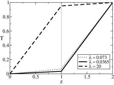
Figure 6. Stationary temperature profiles for λ = 0.073, λ = 0.0365 and λ = 20.
Download figure:
Standard imageFigure 7 shows the marginal Rayleigh number R versus k (the same representation as in figure 3) for different ratios of conductivities λ. The unstable states vanish for λ → 0 or λ → ∞. Further on, the critical wave number kc (and the critical Rayleigh number Rc) depends on λ. Accumulation of these critical points provides the critical line. The minimal Rc is found for λ = 1 with this parameter set. The shapes for λ = 0.0365 and λ = 20 are more or less similar. To show the different nonlinear behavior, we solved the full problem numerically for these two ratios of conductivities with = 0.3.
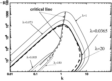
Figure 7. Contour plots of the marginal stability lines in R–k representation. The critical point moves for λ along the critical line. The dashed line is for λ > 1 and the solid line for λ < 1. For λ → 0 and λ → ∞ the system stays stable.
Download figure:
Standard imageIn figure 8, 3D plots of the stationary temperature perturbation fields are shown (with t = 7000). The resolution is 128 × 128 × 20 for each layer and we take an aspect ratio Γ ≈ 42 that corresponds to eight critical modes. For λ = 0.0365 (plot (a)) the stationary patterns are squares and the temperature perturbations are extended into the bulk of the upper fluid. Further on, the temperature perturbations in the upper fluid are 10 times larger than those in the lower fluid, whereas the velocity perturbations are the other way round (not shown). Therefore a strong convective motion occurs basically in the lower layer.

Figure 8. 3D plots for the stationary temperature perturbations for (a) λ = 0.0365 (squares) and (b) λ = 20 (hexagons) with = 0.3, Δt = 0.1 and d = 1. The displayed minimum and maximum temperature perturbations refer to the lower layer and are of the same order for (a) and (b).
Download figure:
Standard imageHowever, for λ = 20 (figure 8(b)) we find hexagonal patterns. The temperature and vertical velocity perturbations are of the same order in both layers. The temperature perturbations are limited to the interface. Furthermore, the absolute value of the velocity perturbations correspond to the velocity perturbations of the upper layer in the former case, i.e. the convective motions in both layers are of the same order as the weak convective motion in the upper layer for λ = 0.0365.
In both situations, the upper layer serves as a heat supplier (α < 1, κ < 1, see the introduction), whereas the underlying convective energy transport fed in the system is fundamentally different and results in different patterns and realized flows.
4. Summary
Anticonvection may appear in two-layer systems via heating from above with buoyancy forces only. This instability mechanism needs a sensitive interaction of bulk and interface forces. At least four timescales must match to yield an anticonvective instability. We have derived the governing equations for the perturbed field quantities. First, we performed a linear stability analysis of the bounded mercury–water system. The linear stability analysis has shown that one unstable k mode is stabilized by further increasing the control parameter −R. Subsequently, we compared vertically bounded with vertically infinitely extended systems. Therefore we derived an analytical expression for the critical Rayleigh number Rc = Rc(k,α,ρ,ν,λ,κ,β1)∝ − k4 in vertically infinitely extended systems. We showed that rigid boundaries lead to an increase of the conductive regime. Subsequently, we presented the fully nonlinear dynamics of an anticonvective system. Hexagons arise for a mercury–water system close to threshold. Increasing the applied temperature gradient leads to a transition to squares. Moreover, two different stationary temperature profiles have revealed how convective heat and mass transport is realized and consequently may influence the resulting stationary patterns. These latter investigations may represent in some way the influence of contaminations or heat sources (sinks) at the interface and provide expectations for experimental setups. Finally, we note that we have not performed an exhaustive investigation of the parameter range for anticonvection due to the amount of parameters (namely at least four) that exceeds our computational facilities. However, experimental results and further theoretical insights may allow for a more restrictive parameter space.
Appendix.: An infinitely extended system
Here we derive an analytical expression for the marginal Rayleigh number Rc of a vertically infinitely extended system. For the sake of simplicity we shift the interface to z = 0 in this section.
The linear equations for the marginal state (equations (14a)–(14d) with growth rate χ = 0) can be written as (e.g. (∂2z − k2) × equation (14a) + Rck2 × equation (14b), see Welander (1964) and Chandrasekhar (1961)):


The six conditions at the interface (see equations (16a) and (16b)) turn out to be


with ε1 = ρν, ε2 = ν/α, ε3 = νλ/α and ε4 = (α/(νκλ))(1/3). Note that β1 is a parameter of the infinitely extended systems and cannot be expressed with equation (7a).
The six roots for fluid 1 (substitute  in equation (A.1a)) are


and for fluid 2 (substitute  in equation (A.1b))


with

and the assumption

that ensures positive arguments of the square roots in equations (A.3) and (A.4).
Since perturbations decay at large distances from the interface, we take into account only the 'active' modes at the interface, i.e. three modes with the positive real part of the roots for fluid 1 and 3 modes with the negative real part of the roots for fluid 2:

This ansatz provides an algebraic system of equations for the amplitudes Cn and Dn with nontrivial solutions det(M) = 0:
After some manipulations we find the second-order surface equation of Welander (1964) in the ε1, ε2 and ε3 space. It can also be written as a quadratic form in the real and imaginary parts of the roots in equations (A.3) and (A.4), namely  .
.

Note that H is symmetric and depends on material parameters alone. The 3 × 3 submatrices can be written as:
with  , h2 = ε34ε2ε3 + ε1, h3 = ε4ε2 and
  .
.
A.1. Conclusions for infinitely extended systems
Firstly, a principal axis transformation of equation (A.8) provides (after back substitution of material parameters)

In general one finds two zero, two negative and two positive eigenvalues. This provides a single sheet hyperboloid in  -space (
  depend on material parameters, whereas
  is independent). For ρ = 1/(κα) one negative eigenvalue becomes zero (rhs of equation (A.9)) and therefore the surface reduces to a cone. We note that a hyperboloid also results directly from equation (A.8) calculating the signature of H (using Sylvester's theorem (Golub and Van Loan 1996)).
Secondly, Welander (1964) has shown that Rc is a monotonic function of k. Therefore we try to extract a simple analytical expression for the marginal Rc from equation (A.8) for large-temperature gradients (i.e. large |Rc|). Equation (A.8) has 17 terms with products of the roots (equations (A.3) and (A.4)). We expand these 17 products of the roots at k = 0 to the order O(k14/3) (i.e. three terms). For the sake of clarity, we present examples of only two of the 17 expanded products:


with  (see equation (A.5)). All expansions underlie the assumptions that, firstly, |Rc| is large (i.e. high orders in k vanish) and, secondly, moderate k values (k < 10) and ε4 > 1 (i.e. expansion at k = 0 is valid). We have checked the validity of these assumptions numerically. The expansion for moderate k values and ε4 > 1 provides a good approximation for the products of the roots (e.g. t1·s1,t1·s2, ...). To exemplify this, we plotted the products and the expansions of equations (A.10a) and (b)) in figure 9 for Rc = −1000. Even this small Rc shows good accordance for k < 4.

Figure 9. The products and the corresponding expansions of the roots from equation (A.10a) are shown for Rc = −1000 and the parameters of table 1. In this case, the expansions are valid for k < 4.
Download figure:
Standard imageSubstituting the 17 expanded products into equation (A.8) and back substitution of  and hi provides, finally, an analytical expression for the marginal Rayleigh number
with
where the proportionality factor C depends on material parameters alone. Note that two solutions exist for Rc in equation (A.11). However, only negative C has a physical meaning, since we restrict ourselves to negative Rayleigh numbers R. Therefore we take the first solution (i.e. ' + ' sign).
Finally, we have compared equation (A.11) with the results of the full 'Welander' equation (A.8). Surprisingly, the marginal stability line is perfectly described by a k4 dependence (even for violating the above-noted assumptions). We mention that the k4 proportionality results already from the expansion to order O(k10/3). However, then the approximation of the coefficient of proportionality C' is no longer valid.